
AI-101 · Lesson 6 of 12 · 26 min
Neural networks and deep learning
Lesson 5 introduced the artificial neuron and showed a single neuron learning the logical AND function. One neuron can only draw a straight line between categories. Stacking many neurons in layers, and training them all together, produces deep neural networks that can learn to recognize faces, translate languages, play games and generate text. Deep learning has driven almost every major AI advance since 2012. This lesson explains how layers create more powerful functions, how networks learn through backpropagation and gradient descent, the main kinds of network and what each is good at, why depth, data and computing power together made the revolution possible, and the practical tricks and limitations that come with these models.
From one neuron to many layers
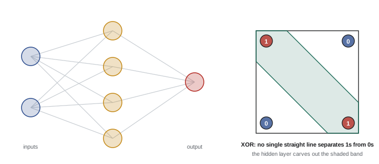
A single neuron draws a straight line (or, in more dimensions, a flat plane) to separate two classes. Many problems cannot be separated that way. The classic example is XOR (exclusive or): output 1 when exactly one input is 1. No single line separates the two 1s from the two 0s. Marvin Minsky and Seymour Papert highlighted this limitation in their 1969 book Perceptrons, which contributed to the first decline in neural network research.
The solution is a hidden layer between inputs and output. Each hidden neuron draws its own line, and the output neuron combines them, so the network can carve out regions of any shape. A network with one large enough hidden layer can approximate any reasonable function (the universal approximation theorem), but in practice deep networks with many layers learn much more efficiently, because each layer builds on the features found by the one before.
Activation functions
Each neuron applies a nonlinear activation function to its weighted sum. Without nonlinearity, any stack of layers would collapse into a single linear function, no more powerful than one neuron. Common activations include the sigmoid, which squashes values into 0 to 1 and is useful for probabilities; tanh, which squashes into −1 to 1; and the rectified linear unit (ReLU), which outputs the input if positive and zero otherwise. ReLU and its variants became standard in deep networks because they are cheap to compute and make deep networks easier to train.
How networks learn: gradient descent and backpropagation
Training adjusts all the weights to make the network's outputs match the desired outputs on training data. As in Lesson 5, this is done by defining a loss (how wrong the network is) and repeatedly nudging every weight in the direction that reduces the loss most steeply, a process called gradient descent. The challenge is computing how the loss changes with respect to each of possibly billions of weights. Backpropagation does this efficiently by applying the chain rule of calculus backward through the network: the error at the output is passed back through each layer, and each weight receives its share of the blame. Popularized by David Rumelhart, Geoffrey Hinton and Ronald Williams in 1986, backpropagation is the engine of all modern deep learning.
where \(\eta\) is the learning rate, which sets the size of each step: too small and training is slow, too large and it overshoots and becomes unstable.
import numpy as np

X = np.array([[0, 0], [0, 1], [1, 0], [1, 1]], dtype=float)
y = np.array([[0], [1], [1], [0]], dtype=float)
rng = np.random.default_rng(2)


def sigmoid(z):
    return 1 / (1 + np.exp(-z))


W1, b1 = rng.normal(0, 1, (2, 4)), np.zeros((1, 4))
W2, b2 = rng.normal(0, 1, (4, 1)), np.zeros((1, 1))
lr = 1.0
for epoch in range(5001):
    h = np.tanh(X @ W1 + b1)
    out = sigmoid(h @ W2 + b2)
    loss = float(np.mean((out - y) ** 2))
    d_out = 2 * (out - y) / len(X) * out * (1 - out)
    d_h = d_out @ W2.T * (1 - h ** 2)
    W2 -= lr * h.T @ d_out
    b2 -= lr * d_out.sum(axis=0, keepdims=True)
    W1 -= lr * X.T @ d_h
    b1 -= lr * d_h.sum(axis=0, keepdims=True)
    if epoch in (0, 100, 500, 1000, 5000):
        print(f"epoch {epoch:>4}: loss {loss:.4f}  outputs {np.round(out.ravel(), 2)}")

w = np.zeros(2); b = 0.0
for _ in range(1000):
    p = sigmoid(X @ w + b)
    g = p - y.ravel()
    w -= 0.5 * X.T @ g / 4
    b -= 0.5 * g.mean()
print("single neuron (no hidden layer):", np.round(sigmoid(X @ w + b), 2))epoch 0: loss 0.2643 outputs [0.5 0.33 0.56 0.41] epoch 100: loss 0.0168 outputs [0.09 0.86 0.87 0.15] epoch 500: loss 0.0014 outputs [0.02 0.96 0.96 0.05] epoch 1000: loss 0.0006 outputs [0.02 0.97 0.97 0.03] epoch 5000: loss 0.0001 outputs [0.01 0.99 0.99 0.01] single neuron (no hidden layer): [0.5 0.5 0.5 0.5]
The output shows the network starting with essentially random guesses and steadily reducing its loss until it outputs nearly 0 for the matching inputs and nearly 1 for the mixed ones. The single neuron, no matter how long it trains, can only output 0.5 for everything, its best compromise given that no straight line works.
Worked problem
Counting parameters
A network for recognizing handwritten digits takes 28 × 28 pixel images (784 inputs), has two hidden layers of 128 and 64 neurons, and 10 outputs. How many weights and biases does it have?
Show solution
- Input to hidden 1: \(784 \times 128 + 128 = 100{,}480\).
- Hidden 1 to hidden 2: \(128 \times 64 + 64 = 8{,}256\).
- Hidden 2 to output: \(64 \times 10 + 10 = 650\).
- Total: \(109{,}386\).
Answer: About 109,000 parameters, all learned from data. Such a network reaches about 98% accuracy on the standard MNIST digit dataset. Large language models have hundreds of billions of parameters, trained by the same basic method at vastly greater scale.
What the layers learn
Deep networks learn hierarchies of features. In an image network, the first layers detect edges and color blobs, middle layers combine them into textures and parts such as eyes or wheels, and later layers respond to whole objects. In a language model, early layers capture word pieces and syntax, and later layers capture meaning, facts and relationships. These features are not programmed; they emerge from training. This is the key difference from earlier approaches, in which engineers designed features by hand.
Main types of networks
- Fully connected (dense) networks: every neuron connects to every neuron in the next layer; good for tabular data and as parts of larger models.
- Convolutional neural networks (CNNs): neurons look at small patches of an image with shared weights, so a feature detector learned in one place works everywhere (Lesson 8). CNNs drove the breakthrough in image recognition in 2012 and remain widely used in vision.
- Recurrent neural networks (RNNs) and LSTMs: process sequences one element at a time with a memory of what came before; long used for speech and translation, now largely replaced by transformers.
- Transformers (2017): use attention, which lets every element of a sequence look directly at every other element and decide what is relevant. Transformers train efficiently on parallel hardware and scale to enormous sizes; they power language models, and increasingly vision, speech and protein models (Lesson 9).
- Generative models: networks that create new data, such as diffusion models for images and video, and language models for text.
| Network type | Key idea | Typical uses |
|---|---|---|
| Dense (fully connected) | Every neuron connected to the next layer | Tabular data, small problems, parts of larger models |
| Convolutional (CNN) | Shared filters scanning local patches | Images, video, medical scans |
| Recurrent (RNN, LSTM) | Memory carried along a sequence | Older speech and text systems, time series |
| Transformer | Attention between all elements | Language models, translation, vision, biology |
| Diffusion model | Learning to remove noise step by step | Image, video and audio generation |
Why deep learning took off after 2012
Neural networks were invented in the 1950s and backpropagation in the 1980s, yet deep learning only took off around 2012. Three things came together:
- Data: the internet produced huge labeled and unlabeled datasets, such as ImageNet's 14 million labeled images (2009).
- Computing power: graphics processing units (GPUs), designed for video games, turned out to be ideal for the matrix multiplications at the heart of neural networks, speeding training by factors of 10 to 100.
- Algorithms and engineering: ReLU activations, better weight initialization, dropout, batch normalization and later residual connections made deep networks trainable, and open-source software (TensorFlow, PyTorch) made them accessible.
In 2012, AlexNet, a CNN trained on two GPUs by Alex Krizhevsky, Ilya Sutskever and Geoffrey Hinton at the University of Toronto, cut the error rate on the ImageNet challenge from about 26% to about 15%, convincing the field. Hinton, along with Yoshua Bengio and Yann LeCun, received the 2018 Turing Award for this work, and Hinton shared the 2024 Nobel Prize in Physics with John Hopfield for foundational discoveries in neural networks.
Worked problem
Why GPUs matter
Training a model requires \(10^{18}\) floating-point operations. A CPU sustains \(10^{12}\) operations per second; a GPU sustains \(4 \times 10^{14}\). How long does each take?
Show solution
- CPU: \(10^{18}/10^{12} = 10^6\) s, about 11.6 days.
- GPU: \(10^{18}/(4 \times 10^{14}) = 2500\) s, about 42 minutes.
Answer: About 12 days on the CPU versus 42 minutes on one GPU, a factor of 400. Today's largest models need around \(10^{25}\) operations or more, which is why they are trained on clusters of tens of thousands of GPUs in specialized data centers.
Overfitting and how to fight it
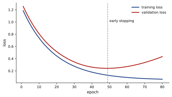
Deep networks have so many parameters that they can memorize training data instead of learning general patterns, performing well on training examples and poorly on new ones (overfitting, Lesson 5). Practitioners use several remedies:
- More data, including data augmentation (flipping, cropping or slightly altering images to create new examples).
- Regularization: penalizing large weights, or dropout, which randomly switches off neurons during training so the network cannot rely on any single one.
- Early stopping: halting training when performance on a separate validation set stops improving.
- Transfer learning: starting from a network pretrained on a large dataset and fine-tuning it on a smaller task, which works remarkably well and is the basis of today's foundation models.
Limitations of deep learning
Deep learning is powerful but has well-known weaknesses:
- Data hunger: many tasks need large amounts of labeled data, which can be expensive or biased.
- Opacity: it is hard to explain why a network made a particular decision, a problem for medicine, finance and law. The field of interpretability tries to understand what networks have learned internally.
- Brittleness: small, carefully chosen changes to an input (adversarial examples) can fool a network, and performance can drop sharply on data unlike the training data.
- Spurious correlations: networks may learn shortcuts, such as recognizing a hospital's scanner label rather than the disease in an X-ray.
- Cost and energy: training and running large models uses significant computing power and electricity.
Understanding these limits is part of using deep learning responsibly (Lessons 10 and 11).
Common mistakes
MistakeThinking more layers always help.
InsteadDeeper networks need more data and careful training; size should match the task.
MistakeUsing linear activations in hidden layers.
InsteadNonlinear activations are essential, or the layers collapse into one.
MistakeJudging a network by training accuracy.
InsteadMeasure performance on held-out validation and test data.
MistakeAssuming a network understands why it is right.
InsteadNetworks can exploit shortcuts; test on varied data.
MistakeTraining from scratch on a small dataset.
InsteadUse transfer learning from a pretrained model.
Summary and key terms
- One neuron draws a straight boundary; hidden layers let networks learn complex functions such as XOR.
- Nonlinear activations (sigmoid, tanh, ReLU) give networks their power.
- Backpropagation computes gradients; gradient descent updates weights: w ← w − η ∂L/∂w.
- Layers learn hierarchies of features automatically.
- CNNs, RNNs, transformers and diffusion models suit different kinds of data.
- Data, GPUs and better algorithms launched deep learning around 2012 (AlexNet).
- Overfitting is fought with more data, regularization, early stopping and transfer learning.
- Deep learning is data-hungry, opaque, sometimes brittle and costly.
- Hidden layer
- A layer of neurons between the input and output layers.
- Activation function
- A nonlinear function applied to a neuron's weighted sum.
- ReLU
- Rectified linear unit: max(0, z).
- Backpropagation
- Computing gradients by applying the chain rule backward through a network.
- Learning rate
- The step size used in gradient descent.
- Convolutional neural network
- A network using shared filters over local patches, suited to images.
- Transformer
- A network architecture based on attention.
- Dropout
- Randomly disabling neurons during training to reduce overfitting.
- Transfer learning
- Adapting a model pretrained on one task to another.
- Adversarial example
- An input altered slightly to fool a model.
Practice problems
Work each problem on paper first, then reveal the answer to check.
Why can't a single neuron learn XOR?
Show answer
XOR is not linearly separable; one neuron draws only a straight boundary.
What would happen if all activations were linear?
Show answer
The whole network would reduce to one linear function.
ReLU of −3 and of 2?
Show answer
0 and 2.
w = 0.8, gradient 0.5, learning rate 0.1. New weight?
Show answer
0.75.
Parameters of a layer with 100 inputs and 20 neurons?
Show answer
100 × 20 + 20 = 2,020.
What do early layers of an image network typically detect?
Show answer
Edges and simple color or texture patterns.
Which network type underlies modern language models?
Show answer
The transformer.
Name the three factors that launched deep learning around 2012.
Show answer
Large datasets, GPUs, improved algorithms and software.
10¹⁹ operations on a GPU at 5 × 10¹⁴ per second. Time?
Show answer
20,000 s, about 5.6 hours.
List three ways to reduce overfitting.
Show answer
More data or augmentation, regularization or dropout, early stopping, transfer learning.
Lesson quiz · 5 questions
Score 60% or more to complete this lesson.
Create a free account to save your progress, take quizzes and earn a certificate.