Search and problem solving

Long before machine learning dominated AI, researchers built programs that solved problems by searching: trying sequences of actions, looking ahead, and choosing the sequence that reaches a goal. Search is still everywhere: route planners find the fastest way home, logistics software schedules deliveries, game programs choose moves, chip designers place components, and the reasoning of modern AI systems often combines learned intuition with explicit search. This lesson introduces the idea of a search problem, compares blind and informed search, shows how programs play games by looking ahead, and explains why many problems are too large to search exhaustively, which is where heuristics and learning come in.

Problems as state spaces

Many problems can be described as a state space:

• States: the possible situations, such as positions on a map, arrangements of a puzzle or configurations of a game board.
• An initial state: where the problem starts.
• Actions: what can be done in each state, such as moving north, sliding a tile or placing a piece.
• A transition model: what state results from each action.
• A goal test: whether a state solves the problem.
• A cost: how expensive each action is, such as distance, time or money.

A solution is a sequence of actions leading from the initial state to a goal; an optimal solution has the lowest total cost. Once a problem is described this way, the same general algorithms can solve route planning, puzzles and scheduling, which is part of what made search such a powerful early idea in AI.

Blind search: breadth-first and depth-first

The simplest search algorithms know nothing about where the goal is. They differ only in the order in which they explore states:

• Breadth-first search (BFS) explores all states one step away, then all states two steps away, and so on. It always finds the shortest solution (in number of steps) but must remember every state at the current depth, which can need enormous memory.
• Depth-first search (DFS) follows one path as deep as possible before backing up and trying another. It needs little memory but can wander down very long or endless paths and does not guarantee the shortest solution.
• Uniform-cost search (the idea behind Dijkstra's algorithm) expands the cheapest path found so far, so it finds the lowest-cost solution when actions have different costs, such as roads of different lengths.

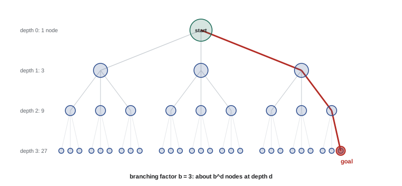
The difficulty is scale. If each state has \(b\) possible actions (the branching factor) and the solution is \(d\) steps away, a blind search may examine about \(b^d\) states. With 10 actions per state and a 10-step solution, that is 10 billion states.

Informed search and heuristics

Informed search uses extra knowledge to explore promising states first. The knowledge comes as a heuristic: an estimate of how far a state is from the goal. For a route on a map, the straight-line distance to the destination is a natural heuristic; for a sliding puzzle, the number of tiles out of place.

The A* algorithm (pronounced "A star", published in 1968) expands the state with the lowest value of

where \(g(n)\) is the cost already spent to reach state \(n\) and \(h(n)\) is the heuristic estimate of the remaining cost. If the heuristic never overestimates the true remaining cost (it is admissible), A* is guaranteed to find an optimal solution, and the better the heuristic, the fewer states it explores. A* and its descendants are used in route planning, robotics, video game characters and many scheduling problems.

from collections import deque
import heapq

grid = [
    "....................",
    "....................",
    "......#########.....",
    "S.............#....G",
    "......#########.....",
    "....................",
    "....................",
]
rows, cols = len(grid), len(grid[0])
start = next((r, c) for r in range(rows) for c in range(cols) if grid[r][c] == "S")
goal = next((r, c) for r in range(rows) for c in range(cols) if grid[r][c] == "G")


def moves(p):
    r, c = p
    for dr, dc in [(1, 0), (-1, 0), (0, 1), (0, -1)]:
        nr, nc = r + dr, c + dc
        if 0 <= nr < rows and 0 <= nc < cols and grid[nr][nc] != "#":
            yield (nr, nc)


def bfs():
    frontier, seen, expanded = deque([(start, 0)]), {start}, 0
    while frontier:
        p, d = frontier.popleft()
        expanded += 1
        if p == goal:
            return d, expanded
        for q in moves(p):
            if q not in seen:
                seen.add(q)
                frontier.append((q, d + 1))


def astar():
    h = lambda p: abs(p[0] - goal[0]) + abs(p[1] - goal[1])
    frontier, best, expanded = [(h(start), 0, start)], {start: 0}, 0
    while frontier:
        f, g, p = heapq.heappop(frontier)
        expanded += 1
        if p == goal:
            return g, expanded
        for q in moves(p):
            if g + 1 < best.get(q, 10 ** 9):
                best[q] = g + 1
                heapq.heappush(frontier, (g + 1 + h(q), g + 1, q))


open_cells = sum(row.count(".") for row in grid) + 2
print("open cells:", open_cells)
print("breadth-first search: path length %d, cells expanded %d" % bfs())
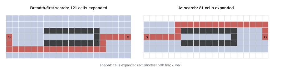
print("A* with Manhattan distance: path length %d, cells expanded %d" % astar())

open cells: 121
breadth-first search: path length 23, cells expanded 121
A* with Manhattan distance: path length 23, cells expanded 81

Both algorithms find the same 23-step path, but A* expands a third fewer cells because its heuristic (the Manhattan distance, counting horizontal and vertical steps to the goal) steers it toward the goal. On larger maps with good heuristics, the savings are often many orders of magnitude.

Playing games: minimax

Games add an opponent who chooses moves to beat you. Adversarial search assumes the opponent plays well. The minimax algorithm looks ahead through possible moves for both players: at your turn you choose the move with the highest value, at the opponent's turn you assume they choose the move with the lowest value for you, and at the end of the game (or at a depth limit) positions are scored as wins, losses, draws or estimated values.

lines = ["XO.", ".X.", "O.."]
board = [c for row in lines for c in row]
WINS = [(0, 1, 2), (3, 4, 5), (6, 7, 8), (0, 3, 6), (1, 4, 7), (2, 5, 8), (0, 4, 8), (2, 4, 6)]
count = 0


def winner(b):
    for a, c, d in WINS:
        if b[a] != "." and b[a] == b[c] == b[d]:
            return b[a]
    return None


def minimax(b, player):
    global count
    count += 1
    w = winner(b)
    if w == "X":
        return 1, None
    if w == "O":
        return -1, None
    moves = [i for i, v in enumerate(b) if v == "."]
    if not moves:
        return 0, None
    best = None
    for m in moves:
        b[m] = player
        score, _ = minimax(b, "O" if player == "X" else "X")
        b[m] = "."
        if best is None or (player == "X" and score > best[0]) or (player == "O" and score < best[0]):
            best = (score, m)
    return best


score, move = minimax(board, "O")
print("O to move. Best move: square", move, "(row", move // 3, "col", move % 3, ")")
print("value with perfect play:", {1: "X wins", 0: "draw", -1: "O wins"}[score])
print("positions examined:", count)
count = 0
minimax(["."] * 9, "X")
print("positions examined from an empty board:", count)

O to move. Best move: square 8 (row 2 col 2 )
value with perfect play: draw
positions examined: 210
positions examined from an empty board: 549946

Even tic-tac-toe has over half a million positions in its full game tree. Chess has an estimated \(10^{120}\) possible games, far too many to search. Game programs therefore search to a limited depth, estimate the value of positions with an evaluation function, and prune branches that cannot affect the decision (alpha-beta pruning, which can cut the work roughly to the square root). IBM's Deep Blue, which beat world champion Garry Kasparov in 1997, searched about 200 million positions per second using hand-crafted evaluation functions.

Combining search with learning

For the game of Go, with roughly 250 legal moves per position and games of about 150 moves, brute-force search was hopeless and hand-written evaluation functions were poor. DeepMind's AlphaGo (2016) combined Monte Carlo tree search, which samples promising lines of play rather than searching all of them, with deep neural networks that learned to suggest good moves and to evaluate positions from millions of games. AlphaZero (2017) then learned chess, shogi and Go from scratch by playing against itself, reaching superhuman strength in each within hours of training on powerful hardware.

The same combination of learned intuition and explicit search appears in modern AI more broadly: reasoning models generate and check multiple lines of thought; code-generating systems test candidate programs; and scientific tools such as AlphaFold and materials discovery systems search vast spaces guided by learned models.

Constraint satisfaction and optimization

Some problems are not about finding a path but about finding an assignment that satisfies constraints: scheduling exams so no student has two at once, assigning frequencies to radio towers, or filling in a Sudoku. Constraint satisfaction algorithms assign values one variable at a time, check constraints immediately, and backtrack when a choice leads to a dead end; techniques such as constraint propagation (eliminating impossible values early) make them very effective in practice.

Other problems seek the best solution among many acceptable ones: the shortest delivery route through 100 stops (the traveling salesperson problem), the cheapest power plant schedule, or the most efficient layout of a factory. When exact search is too expensive, local search methods start from a reasonable solution and improve it step by step (hill climbing), sometimes accepting worse moves to escape local optima (simulated annealing), or evolve a population of solutions (genetic algorithms). These methods rarely guarantee the best answer but often find very good ones quickly.

What search teaches about AI

Search shows several ideas that recur throughout AI. Representing a problem well is half the work. Exhaustive approaches fail on realistic problems because of exponential growth, so intelligent systems need knowledge, heuristics or learned intuition to focus their effort. And a system can be superhuman in a narrow, well-defined domain such as chess while having no understanding of anything outside it. Lesson 4 turns to another classic approach: representing knowledge explicitly and reasoning with it, including under uncertainty.