
AERO-440 · Lesson 9 of 12 · 26 min
Turbulence modeling
Every RANS result the group produces rests on a turbulence model, and the choice of model is the largest single physical assumption in the calculation. When Sam Littlechild, the test pilot, asks why the CFD stall angle for the Tern Block 2 changed by two degrees between two runs of the same geometry, the answer turns out to be that one run used the Spalart-Allmaras model and the other the SST model. Tomasz decides that everyone in the group, and anyone who reads its reports, should understand what these models are, where they came from, and when they can be believed. This lesson provides that understanding.
Reynolds averaging
Turbulent flow is unsteady and three-dimensional at scales from the size of the body down to fractions of a millimeter. For engineering, the mean flow is usually what matters. Osborne Reynolds proposed in 1895 to split each variable into a mean and a fluctuation, \(u_i = \bar{u}_i + u_i'\), and to average the equations. For compressible flow, a density-weighted average, due to Favre, keeps the averaged equations tidy. The averaged momentum equation contains a new term, the Reynolds stress \(-\rho\,\overline{u_i' u_j'}\), which represents the transport of momentum by the turbulent fluctuations.
The Reynolds stress adds six unknowns and no new equations. This is the closure problem of turbulence. Exact equations for the Reynolds stresses can be derived, but they contain still higher correlations, and the hierarchy never closes. A turbulence model supplies the missing relation, using a mixture of physical reasoning, dimensional analysis and calibration against experiments.
The eddy-viscosity hypothesis
Most engineering models use Joseph Boussinesq's hypothesis of 1877: the Reynolds stress behaves like an additional viscous stress, proportional to the mean strain rate, with a turbulent or eddy viscosity \(\mu_t\) in place of the molecular viscosity.
Here \(k\) is the turbulent kinetic energy. The task of the model is reduced to finding one scalar, the eddy viscosity, at every point. The hypothesis is good in thin shear layers, such as attached boundary layers, where one component of strain dominates. It is poor where the turbulence is strongly anisotropic or where the stress does not follow the strain: in strongly curved or rotating flows, in corner flows such as a wing-fuselage junction, and in regions of sudden strain change. Unlike the molecular viscosity, the eddy viscosity is a property of the flow, not of the fluid, and in a boundary layer it can exceed the molecular value by a factor of a hundred or more.
Algebraic models: mixing length
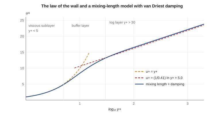
The simplest models give the eddy viscosity algebraically. Ludwig Prandtl's mixing-length model of 1925 sets \(\nu_t = \ell^{2}|\partial u/\partial y|\), with a mixing length \(\ell\) proportional to the distance from the wall, \(\ell = \kappa y\), where \(\kappa \approx 0.41\) is the von Kármán constant. Very close to the wall, turbulence is damped by viscosity, and Edward van Driest's damping function, \(\ell = \kappa y(1 - e^{-y^{+}/A^{+}})\) with \(A^{+} \approx 26\), reduces the mixing length smoothly to zero. The Cebeci-Smith and Baldwin-Lomax models of the 1970s extended this to complete boundary layers with an outer-layer formulation; Baldwin-Lomax was the workhorse of early Navier-Stokes codes because it needed no extra equations.
The near-wall region of a turbulent boundary layer has a universal structure, the law of the wall, expressed in wall units \(u^{+} = \bar{u}/u_{\tau}\) and \(y^{+} = y u_{\tau}/\nu\). In the viscous sublayer, \(y^{+} < 5\), \(u^{+} = y^{+}\). In the log layer, beyond about \(y^{+} = 30\), \(u^{+} = (1/\kappa)\ln y^{+} + B\), with \(B \approx 5.0\). Between them is the buffer layer. A model that integrates to the wall must reproduce this structure. The code below integrates the momentum balance across a constant-stress inner layer for two eddy-viscosity models and compares the result with the log law.
# Inner layer of a turbulent wall flow with constant total shear stress (tau = tau_w):
#   (1 + nu_t/nu) du+/dy+ = 1.
# Model A: Prandtl mixing length with van Driest damping, l+ = kappa y+ (1 - exp(-y+/26)).
# Model B: the Spalart-Allmaras near-wall form, nu_t/nu = chi * fv1(chi) with chi = kappa y+ (its log-layer solution).
import math
kappa, A = 0.41, 26.0
def lplus(yp):
    return kappa * yp * (1 - math.exp(-yp / A))
def dudy_ml(yp):
    # with constant stress, nu_t+ = l+^2 du+/dy+; solving the quadratic gives du+/dy+ directly
    l = lplus(yp)
    return 2 / (1 + math.sqrt(1 + 4 * l * l))
def dudy_sa(yp):
    chi = kappa * yp; fv1 = chi**3 / (chi**3 + 7.1**3)
    return 1 / (1 + chi * fv1)
def integrate(dudy, ys):
    u, out, y, k = 0.0, {}, 0.0, 0
    h = 0.01
    while y < ys[-1] - 1e-12:
        step = min(h * (1 + y), ys[k] - y)              # coarser steps far from the wall
        u += step / 6 * (dudy(y) + 4 * dudy(y + step / 2) + dudy(y + step))
        y += step
        if abs(y - ys[k]) < 1e-9:
            out[ys[k]] = u; k += 1
    return out
ys = [1, 5, 10, 30, 100, 300, 1000]
ml, sa = integrate(dudy_ml, ys), integrate(dudy_sa, ys)
print("   y+    u+ mixing length   u+ SA form   log law 2.44 ln y+ + 5.0")
for y in ys:
    log = math.log(y) / kappa + 5.0
    print(f"{y:6d}       {ml[y]:7.2f}         {sa[y]:7.2f}        {log:7.2f}" + ("   (viscous sublayer: u+ = y+)" if y < 5 else ""))
B_ml = ml[1000] - math.log(1000) / kappa
B_sa = sa[1000] - math.log(1000) / kappa
print(f"Implied log-law intercept B: mixing length {B_ml:.2f}, SA form {B_sa:.2f} (measured flows: about 5.0 to 5.2)")
yp = 100
print(f"Eddy-to-molecular viscosity ratio at y+ = 100: mixing length {lplus(yp)**2 * dudy_ml(yp):.1f}, "
f"SA {kappa*yp*(kappa*yp)**3/((kappa*yp)**3 + 7.1**3):.1f}") y+ u+ mixing length u+ SA form log law 2.44 ln y+ + 5.0
1 1.00 1.00 5.00 (viscous sublayer: u+ = y+)
5 4.88 4.95 8.93
10 8.42 8.95 10.62
30 13.19 13.38 13.30
100 16.53 16.32 16.23
300 19.20 18.96 18.91
1000 22.13 21.89 21.85
Implied log-law intercept B: mixing length 5.28, SA form 5.04 (measured flows: about 5.0 to 5.2)
Eddy-to-molecular viscosity ratio at y+ = 100: mixing length 39.6, SA 40.8Both models give \(u^{+} = y^{+}\) at the wall and the log law far from it. The mixing-length model with van Driest's damping gives an intercept \(B = 5.28\), and the Spalart-Allmaras form gives 5.04; measured flows give about 5.0 to 5.2. Both models were calibrated to do this, so the agreement confirms that the code and the models are consistent rather than that the models are right in general. The eddy viscosity at \(y^{+} = 100\) is about 40 times the molecular viscosity in both models, which is why turbulent boundary layers are thicker and have higher skin friction than laminar ones.
One-equation models: Spalart-Allmaras
Algebraic models cannot carry the history of the turbulence: a boundary layer that has passed through an adverse pressure gradient is different from one that has not. Transport-equation models solve partial differential equations for turbulence quantities so that turbulence can be convected and diffused. The Spalart-Allmaras model, published by Philippe Spalart and Steven Allmaras in 1992, solves one transport equation for a working variable \(\tilde{\nu}\) related to the eddy viscosity by \(\nu_t = \tilde{\nu} f_{v1}\), with \(f_{v1} = \chi^{3}/(\chi^{3} + c_{v1}^{3})\), \(\chi = \tilde{\nu}/\nu\) and \(c_{v1} = 7.1\). The equation contains production, destruction based on wall distance, and diffusion terms, calibrated against simple flows. It was designed for aerodynamic flows, is robust and inexpensive, and is the most widely used model in aircraft external aerodynamics. It is the default model of the AIAA Drag Prediction Workshops and of many company practices, including the group's.
Two-equation models
Two-equation models solve for two turbulence quantities, from which a velocity scale and a length scale, and hence an eddy viscosity, follow. The \(k\)-\(\varepsilon\) model, with turbulent kinetic energy and its dissipation rate, gives \(\nu_t = C_\mu k^{2}/\varepsilon\) and works well in free shear flows, but it needs wall functions or damping functions near walls and predicts separation too late in adverse pressure gradients. Wilcox's \(k\)-\(\omega\) model, with the specific dissipation rate \(\omega\), integrates to the wall without damping and handles adverse pressure gradients better, but its results depend on the freestream value of \(\omega\). Florian Menter's shear stress transport model, SST, of 1994 blends the two: \(k\)-\(\omega\) near the wall, \(k\)-\(\varepsilon\) away from it, with a limiter on the eddy viscosity that respects the observed relation between shear stress and turbulent kinetic energy in adverse pressure gradients. SST predicts the onset of separation better than most eddy-viscosity models and is the most common two-equation model in aerospace.
| Model | Equations | Strengths | Known weaknesses |
|---|---|---|---|
| Baldwin-Lomax | 0 | Cheap, no extra equations | Poor for separation and wakes; no history |
| Spalart-Allmaras | 1 | Robust, accurate for attached airfoil and wing flows | Separation onset and corner flows; free shear layers |
| \(k\)-\(\varepsilon\) | 2 | Free shear flows | Needs wall treatment; late separation prediction |
| \(k\)-\(\omega\) (Wilcox) | 2 | Integrates to the wall | Sensitive to freestream \(\omega\) |
| SST (Menter) | 2 | Better separation onset; widely validated | Can predict separation too early in some flows |
| Reynolds stress models | 6 or 7 | Anisotropy, curvature, corners | Costly; less robust |
Transition
Standard RANS models assume the boundary layer is turbulent everywhere, or they let the model decide, which it does poorly. On the Tern Block 2 wing, the laminar run of the boundary layer changes the skin friction by several counts and affects the trailing-edge separation near stall. Transition models address this. The \(\gamma\)-\(Re_\theta\) model of Langtry and Menter adds two transport equations, for intermittency and a transition-onset Reynolds number, and uses empirical correlations for natural and bypass transition; simpler one-equation versions also exist. Engineers can instead specify the transition location from experiments or from a stability analysis such as the \(e^{N}\) method. The group's practice is to run fully turbulent for robustness and conservatism, and to add a transition model, or a specified trip, when skin friction or maximum lift must be matched closely.
Beyond RANS: hybrid methods and LES
For massively separated flows, RANS models fail in principle: the large eddies in a separated region are not universal and cannot be averaged away. Detached-eddy simulation, proposed by Spalart and colleagues in 1997, uses RANS in attached boundary layers and switches to an LES-like mode where the grid is fine enough to resolve large eddies. Variants such as delayed DES and improved delayed DES protect the boundary layer from a premature switch. Wall-modeled LES resolves the outer boundary layer and models the inner layer. These methods cost one or two orders of magnitude more than RANS and need time-accurate runs, but they are increasingly used for high-lift and buffet problems, and the High Lift Prediction Workshops have included them.
Where to find the truth: the Turbulence Modeling Resource
Implementing a turbulence model correctly is harder than it looks: published papers contain typographical errors, variants proliferate, and small differences in wall-distance or limiter details change results. the NASA Turbulence Modeling Resource, created at NASA Langley and now maintained with the AIAA Turbulence Model Benchmarking Working Group, documents the standard forms of models such as Spalart-Allmaras and SST, and provides verification cases, such as a flat plate and a two-dimensional bump, with grid families and reference results from independent codes. The group verifies its implementation against these cases before running any aircraft, and names the model variant precisely in every report, for example SA-noft2, the Spalart-Allmaras model without the trip term \(f_{t2}\).
Worked problem
Eddy viscosity in the log layer
For the Tern Block 2 at cruise, \(u_\tau = 3.8\ \mathrm{m/s}\) and \(\nu = 1.9 \times 10^{-5}\ \mathrm{m^2/s}\). Estimate the eddy viscosity at \(y = 0.5\ \mathrm{mm}\) using \(\nu_t = \kappa u_\tau y\).
Show solution
- \(y^{+} = 3.8 \times 0.0005/1.9 \times 10^{-5} = 100\): in the log layer.
- \(\nu_t = 0.41 \times 3.8 \times 0.0005 = 7.8 \times 10^{-4}\ \mathrm{m^2/s}\).
- Ratio to \(\nu\): about 41.
Answer: About \(7.8 \times 10^{-4}\ \mathrm{m^2/s}\), roughly 40 times the molecular value, as the code found.
Worked problem
Choosing a model for the nacelle
The Petrel 19 nacelle afterbody has a mild adverse pressure gradient that may separate at climb power. Marcus needs a load estimate. Which model should the group use first, and what check should follow?
Show solution
- Spalart-Allmaras is robust but tends to predict separation late.
- SST predicts separation onset better in adverse pressure gradients.
- Running both brackets the model uncertainty; if they disagree, a hybrid method or test is needed.
Answer: Run SST and Spalart-Allmaras; use the spread as a measure of model uncertainty, and flag the case for tunnel or DES work if the difference is large.
Worked problem
Log law velocity
What is \(u^{+}\) at \(y^{+} = 300\) from the log law with \(\kappa = 0.41\) and \(B = 5.0\)?
Show solution
- \(u^{+} = (1/0.41)\ln 300 + 5.0\).
- \(\ln 300 = 5.70\), so \(u^{+} = 13.91 + 5.0 = 18.91\).
Answer: 18.91, matching the code's log-law column.
Common mistakes
MistakeThe turbulence model only matters for separated flows.
InsteadIt sets skin friction and boundary-layer growth everywhere, and so affects drag and shock position even in attached flow.
MistakeTwo-equation models are always more accurate than one-equation models.
InsteadFor attached aerodynamic flows, Spalart-Allmaras is often as accurate as SST; more equations do not guarantee better physics.
MistakeThe eddy viscosity is a property of air.
InsteadIt is a property of the turbulent flow and varies through the boundary layer.
MistakeModel names identify the model exactly.
InsteadMany variants exist; reports must name the exact variant, as the NASA Turbulence Modeling Resource recommends.
Summary and key terms
- Reynolds averaging introduces the Reynolds stress and the closure problem.
- The Boussinesq hypothesis replaces the Reynolds stress with an eddy viscosity, good in thin shear layers but poor in strongly anisotropic flows.
- Mixing-length models with van Driest damping reproduce the law of the wall.
- The Spalart-Allmaras one-equation model is the standard for aircraft external aerodynamics, and Menter's SST is the most common two-equation model.
- Transition models, hybrid RANS-LES and LES extend the range at higher cost, and the NASA Turbulence Modeling Resource provides standard model forms and verification cases.
- Reynolds stress
- The averaged product of velocity fluctuations, acting as an extra stress on the mean flow.
- Closure problem
- The averaged equations contain more unknowns than equations.
- Eddy viscosity
- A turbulent viscosity relating Reynolds stress to mean strain.
- Law of the wall
- The universal near-wall velocity profile in wall units.
- Spalart-Allmaras model
- A one-equation eddy-viscosity model designed for aerodynamic flows.
- SST model
- Menter's blend of k-omega near walls and k-epsilon away from them, with a shear-stress limiter.
- Detached-eddy simulation
- A hybrid method using RANS in boundary layers and LES in separated regions.
Practice problems
Work each problem on paper first, then reveal the answer to check.
What is \(y^{+}\) at which the log law is usually taken to begin?
Show answer
About 30.
In the SA model, what is \(f_{v1}\) when \(\chi = 7.1\)?
Show answer
\(7.1^3/(2 \times 7.1^3) = 0.5\).
Why does the \(k\)-\(\omega\) model need care with freestream values?
Show answer
Its results depend on the freestream value of \(\omega\).
Name one flow feature where the Boussinesq hypothesis is poor.
Show answer
Corner flow at a wing-fuselage junction, or strongly curved or rotating flow.
Why does the group run fully turbulent by default?
Show answer
For robustness and conservatism; transition modeling adds uncertainty and is used when friction or maximum lift must be matched.
Lesson quiz · 5 questions
Score 60% or more to complete this lesson.
Create a free account to save your progress, take quizzes and earn a certificate.