
AERO-440 · Lesson 11 of 12 · 26 min
Airfoil and wing case studies
With a verified solver and a validated practice for cruise drag, the group turns to the questions the programs are actually asking. This lesson follows four case studies through the group's first year: the Tern Block 2 root section across its lift range, the Swift 900 wing at transonic cruise, the Petrel 19 nacelle and wing junction, and the Tern Block 2 in its landing configuration. Each shows a different side of what CFD does well, what it does poorly, and how the group combined it with theory and test to reach a decision.
Case 1: the Tern Block 2 root section
The Tern Block 2 wing uses a NACA 4415 section at the root and a 4412 at the tip, both with the same 4 percent camber line. Thin-airfoil theory, from the first aerodynamics course, gives a lift-curve slope of \(2\pi\) per radian and a zero-lift angle of about \(-4.15^\circ\) for this camber line, independent of thickness and Reynolds number. Before running RANS, Arjun builds the simplest discrete method that reproduces thin-airfoil theory: the lumped-vortex method. The camber line is divided into panels, a point vortex is placed at the quarter-point of each, and the flow tangency condition is enforced at the three-quarter point. The result is a small linear system for the vortex strengths, whose sum gives the lift.
# Lumped-vortex (discrete vortex) method on the NACA 4415 camber line, compared with thin-airfoil theory,
# then set beside RANS and wind-tunnel values for the Tern Block 2 root section (illustrative numbers).
import math
m, p = 0.04, 0.4                                       # NACA 4415: 4 % camber at 40 % chord
def zc(x):  return m / p**2 * (2*p*x - x*x) if x < p else m / (1-p)**2 * (1 - 2*p + 2*p*x - x*x)
def solve(alpha_deg, n):
    a = math.radians(alpha_deg)
    xs = [0.5 * (1 - math.cos(math.pi * k / n)) for k in range(n + 1)]      # cosine spacing
    pts = [(x, zc(x)) for x in xs]
    vort, ctrl, nrm = [], [], []
    for k in range(n):
        (x0, z0), (x1, z1) = pts[k], pts[k + 1]
        dx, dz = x1 - x0, z1 - z0; L = math.hypot(dx, dz)
        vort.append((x0 + 0.25*dx, z0 + 0.25*dz)); ctrl.append((x0 + 0.75*dx, z0 + 0.75*dz))
        nrm.append((-dz / L, dx / L))
    A = [[0.0]*n for _ in range(n)]; b = [0.0]*n
    for i, (xc, zc_) in enumerate(ctrl):
        for j, (xv, zv) in enumerate(vort):           # induced velocity of a unit clockwise vortex
            rx, rz = xc - xv, zc_ - zv; r2 = rx*rx + rz*rz
            u, w = rz / (2*math.pi*r2), -rx / (2*math.pi*r2)
            A[i][j] = u * nrm[i][0] + w * nrm[i][1]
        b[i] = -(math.cos(a) * nrm[i][0] + math.sin(a) * nrm[i][1])
    for c in range(n):                                # Gaussian elimination with partial pivoting
        r = max(range(c, n), key=lambda q: abs(A[q][c])); A[c], A[r] = A[r], A[c]; b[c], b[r] = b[r], b[c]
        for q in range(c + 1, n):
            fct = A[q][c] / A[c][c]; b[q] -= fct * b[c]
            for k in range(c, n): A[q][k] -= fct * A[c][k]
    g = [0.0]*n
    for c in range(n - 1, -1, -1): g[c] = (b[c] - sum(A[c][k]*g[k] for k in range(c + 1, n))) / A[c][c]
    return 2 * sum(g)                                  # cl = 2 * Gamma / (V c) with V = c = 1
th = lambda al: 2*math.pi*math.radians(al + 4.15)     # thin-airfoil result for the 4415 camber line
print(f"Lumped-vortex cl at 4 deg against the number of panels (thin-airfoil value {th(4):.4f})")
for n in (10, 20, 40, 80):
    print(f"  {n:2d} panels: cl = {solve(4, n):.4f}")
c0, c8 = solve(0, 80), solve(8, 80)
slope = (c8 - c0) / 8; aL0 = -c0 / slope
print(f"80 panels: slope {slope:.4f} per deg ({slope*180/math.pi:.3f} per rad), zero-lift angle {aL0:.2f} deg")
print()
rows = (("thin airfoil / lumped vortex", slope, aL0, solve(4, 80), None),
        ("RANS (SA, fully turbulent)", 0.1065, -3.9, 0.840, 1.62),
        ("RANS (SST, transition model)", 0.1072, -4.0, 0.856, 1.68),
        ("wind tunnel, Re 3 million", 0.1060, -4.0, 0.845, 1.66))
print("method                          slope/deg  alpha_L0  cl at 4 deg  cl,max")
for name, s, a0, c4, cmax in rows:
    print(f"{name:31s} {s:8.4f}   {a0:6.2f}     {c4:6.3f}     " + ("  --" if cmax is None else f"{cmax:.2f}"))
print(f"Thin theory overpredicts cl at 4 deg by {100*(solve(4,80)/0.845 - 1):.0f} % against the tunnel value")Lumped-vortex cl at 4 deg against the number of panels (thin-airfoil value 0.8937) 10 panels: cl = 0.8485 20 panels: cl = 0.8707 40 panels: cl = 0.8815 80 panels: cl = 0.8869 80 panels: slope 0.1088 per deg (6.236 per rad), zero-lift angle -4.13 deg method slope/deg alpha_L0 cl at 4 deg cl,max thin airfoil / lumped vortex 0.1088 -4.13 0.887 -- RANS (SA, fully turbulent) 0.1065 -3.90 0.840 1.62 RANS (SST, transition model) 0.1072 -4.00 0.856 1.68 wind tunnel, Re 3 million 0.1060 -4.00 0.845 1.66 Thin theory overpredicts cl at 4 deg by 5 % against the tunnel value
With 80 panels, the lumped-vortex method gives a slope of 6.24 per radian and a zero-lift angle of \(-4.13^\circ\), within 1 percent of thin-airfoil theory, and the lift at \(4^\circ\) approaches the theoretical 0.894 as panels are added. The RANS and tunnel values in the table are representative of what the group obtained for the section at a Reynolds number of 3 million; they are illustrative rather than published data. All methods agree on the zero-lift angle within about a quarter of a degree. The slope from RANS and from the tunnel is about 2 to 3 percent below the thin-airfoil value, because the boundary layer thickens on the upper surface and decambers the section, so thin theory overpredicts \(c_l\) at \(4^\circ\) by about 5 percent.
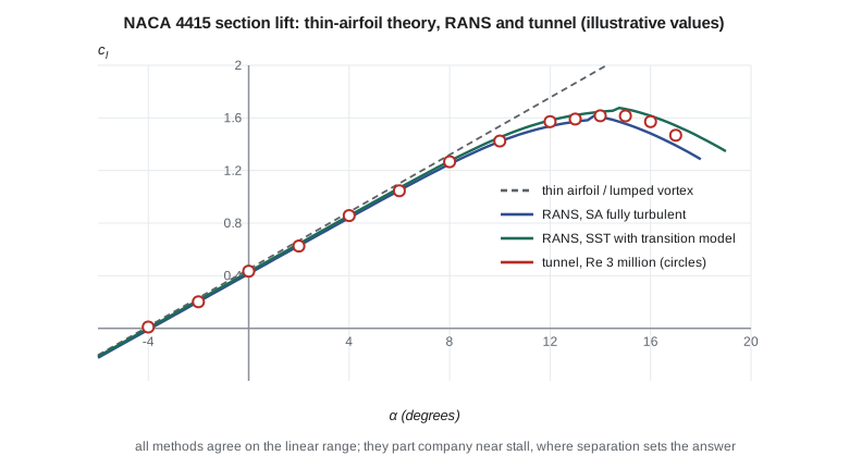
Near stall, the story changes. The fully turbulent Spalart-Allmaras run gives a maximum lift coefficient of 1.62; the SST run with a transition model gives 1.68; the tunnel gives 1.66. The spread of 0.06 is small in absolute terms but corresponds to about two degrees of stall angle, the difference Sam noticed in lesson 9. More important is the shape of the curve beyond the peak. On a thick, cambered section like the 4415, stall is trailing-edge stall: separation starts at the trailing edge and moves forward gradually, giving a rounded peak. Both RANS models capture this qualitatively, but the post-stall lift depends on details of the separated flow that steady RANS cannot represent well. The group's practice is to report RANS maximum lift with a stated uncertainty of about 0.1 in \(c_l\) and to use tunnel data for any number that goes into performance or handling calculations.
Case 2: the Swift 900 transonic wing
Kenji's high-speed group has chosen a supercritical section for the Swift 900, with 25 degrees of quarter-chord sweep and a mean thickness ratio of 12 percent. At the cruise Mach number of 0.80, a pocket of supersonic flow forms over the upper surface and ends in a shock. The design aim is a weak shock, with a peak Mach number ahead of it not much above 1.2, so that wave drag is small and the boundary layer does not separate at the shock foot. RANS with Spalart-Allmaras, on grids adapted to the shock, is run from Mach 0.70 to 0.84 at the design lift coefficient.
Three features of the results matter. First, the shock position is very sensitive: a change of one hundredth in Mach number moves the shock several percent of chord, and the turbulence model, through the boundary-layer thickness at the shock, moves it as much again. Second, the drag-divergence Mach number, defined here as the Mach number where \(dC_D/dM = 0.1\), comes out at 0.83 from CFD, close to the estimate of about 0.84 from the Korn equation used in the compressible-flow course. Third, at Mach 0.84 and a lift coefficient 0.1 above the design value, the RANS solution shows a small separation bubble behind the shock and does not converge to a steady state. That is a sign of approaching buffet, the unsteady shock oscillation that sets the upper limit of the cruise envelope. Steady RANS can indicate buffet onset by the appearance of shock-induced separation, but predicting the buffet itself needs unsteady RANS or hybrid methods and, ultimately, test data.
| Quantity | CFD (RANS, SA) | Remark |
|---|---|---|
| Peak Mach number ahead of the shock at Mach 0.80 | 1.19 | Weak shock as designed |
| Shock position at Mach 0.80, mid-span | 58 percent chord | Moves about 4 percent chord per 0.01 Mach |
| Drag-divergence Mach number | 0.83 | Close to the Korn estimate of about 0.84 |
| Wave drag at Mach 0.80 | about 4 counts | Small, as intended |
| Shock-induced separation onset | Mach 0.84 at design lift + 0.1 | Indicates approaching buffet |
Case 3: the Petrel 19 nacelle and wing
The Petrel 19 has a high wing with two nacelles for its electric motors, each driving a large propeller. Marcus needs pressure loads on the nacelles for the structure, and Élise needs the interference drag to close the drag estimate from the conceptual design. Here RANS is in its element: the flow is attached, the question is about increments, and components can be added and removed at will, something no tunnel test can do as cleanly.
The group runs three configurations at the cruise condition: clean wing and fuselage, wing and fuselage with nacelles, and the same with the nacelles moved 150 mm forward. The nacelles add 14 counts of drag, of which about 4 counts is interference, mostly from the junction where the nacelle meets the wing's lower surface. Moving them forward reduces the interference by about 1.5 counts, because the nacelle's pressure field then overlaps less with the wing's pressure recovery. The propeller slipstream is modeled with an actuator disk, which adds momentum and swirl over the propeller disk area without resolving the blades; this gives the time-averaged effect of the slipstream on wing loading, which raises the local lift behind each propeller by up to 15 percent at climb power. The group stresses that the increments are more reliable than the absolute values, in line with the workshop findings in lesson 10.
Case 4: the Tern Block 2 in landing configuration
The final case is the hardest. The Tern Block 2 landing configuration has double-slotted Fowler flaps, and the program wants to know whether a small change to the flap gap will raise maximum lift. High-lift flows contain everything that makes CFD difficult: confluent boundary layers, with the wakes of the main element and the forward flap vane passing over the aft flap, strong adverse pressure gradients, transition on each element, and separation that grows rapidly near the maximum. The AIAA High Lift Prediction Workshops have shown wide scatter in predicted maximum lift between participants for such configurations, and sensitivity to grids, models and even to whether the solution is run steady or time-accurate.
The group's approach is cautious. It uses CFD for trends at angles well below stall, where the flow is attached and RANS is reliable: the change in lift at a fixed angle when the gap is changed, and the pressure distribution on the flap. It then uses these trends to choose two gap settings for the tunnel. RANS predicts that the narrower gap raises lift at \(8^\circ\) by 0.04 and delays flap trailing-edge separation; the tunnel confirms a gain in maximum lift of 0.05, slightly more than the CFD increment at \(8^\circ\). The CFD did not predict maximum lift itself, but it picked the right configuration to test.
Lessons across the cases
Across the four cases, a pattern emerges that matches industry experience. CFD is most reliable for attached flows, for pressure distributions and for increments between similar configurations. It is useful but must be checked for transonic shock positions and drag rise. It is least reliable for maximum lift, buffet and post-stall behavior, where separation dominates. In every case, the group's confidence came from understanding the physics well enough to know which regime it was in, and from comparison with theory or test at a known point.
Worked problem
Thin-airfoil lift
Find the thin-airfoil lift coefficient of the NACA 4415 at \(4^\circ\), with \(\alpha_{L0} = -4.15^\circ\).
Show solution
- \(c_l = 2\pi(\alpha - \alpha_{L0})\) with angles in radians.
- \(\alpha - \alpha_{L0} = 8.15^\circ = 0.1422\ \mathrm{rad}\).
- \(c_l = 2\pi \times 0.1422 = 0.894\).
Answer: 0.894, the value the lumped-vortex method approaches as panels are added.
Worked problem
Shock movement and Mach uncertainty
The Swift 900 shock moves about 4 percent of chord per 0.01 in Mach number. If the tunnel's Mach number is uncertain by \(\pm 0.003\), how much shock-position uncertainty does that alone cause?
Show solution
- \(0.003/0.01 \times 4 = 1.2\) percent chord.
- With the 2.4 m mean chord used in lesson 6, this is about 29 mm.
Answer: About 1.2 percent of chord. Comparisons of transonic shock position must include Mach number uncertainty in \(u_{\text{input}}\).
Worked problem
Interference drag fraction
The nacelles add 14 counts, of which 4 counts is interference. The Petrel 19 zero-lift drag coefficient from the concept design is 0.0240, or 240 counts. What share of that does interference represent, and is it worth pursuing?
Show solution
- \(4/240 = 1.7\) percent of cruise drag.
- Moving the nacelles forward recovers 1.5 counts, about 0.6 percent.
- On a commuter flying many short legs, 0.6 percent in cruise drag affects fuel and battery energy measurably, if the structural and balance penalties are small.
Answer: About 1.7 percent of the zero-lift drag; the 1.5-count gain is worth carrying into the trade study if the structure and balance allow it.
Common mistakes
MistakeRANS maximum lift can be used directly in performance calculations.
InsteadMaximum lift depends on separation and transition; use tunnel or flight data for performance, with RANS for trends.
MistakeA steady RANS solution that does not converge has a numerical problem.
InsteadIt may be capturing real unsteadiness, such as approaching buffet or stall, which needs time-accurate methods.
MistakeThin-airfoil theory is obsolete now that RANS is available.
InsteadIt gives the linear lift range within a few percent in seconds, and is a valuable check on RANS.
MistakeAbsolute nacelle drag from CFD is as reliable as the increment.
InsteadErrors common to both configurations cancel in increments, which are more reliable than absolute values.
Summary and key terms
- The lumped-vortex method reproduces thin-airfoil theory and agrees with RANS and tunnel data in the linear range.
- Near stall, turbulence models and tests diverge, so maximum lift is taken from tests.
- Transonic RANS predicts shock position, drag rise and the onset of shock-induced separation, with high sensitivity to Mach number and turbulence model.
- RANS is at its best for attached-flow increments such as nacelle interference, and in high-lift work it is used for trends that choose what to test.
- Knowing which flow regime a case is in is the key to knowing how far to trust it.
- Lumped-vortex method
- A discrete vortex method on the camber line with vortices at panel quarter-points and control points at three-quarter points.
- Trailing-edge stall
- Stall in which separation begins at the trailing edge and moves forward gradually.
- Drag divergence
- The rapid rise of drag with Mach number as shocks strengthen.
- Buffet
- Unsteady shock oscillation and separation that limits the cruise envelope.
- Actuator disk
- A model of a propeller as a disk adding momentum and swirl, without resolving blades.
- Interference drag
- Extra drag from the interaction of components beyond the sum of their isolated drags.
- Confluent boundary layer
- A boundary layer merging with the wake of an upstream element in a multi-element wing.
Practice problems
Work each problem on paper first, then reveal the answer to check.
Why is the zero-lift angle of the 4415 and 4412 the same in thin-airfoil theory?
Show answer
They share the same camber line, and thin-airfoil theory depends only on camber.
What lift-curve slope does thin-airfoil theory give per degree?
Show answer
\(2\pi/57.3 = 0.1097\) per degree.
Why does the boundary layer reduce the lift-curve slope?
Show answer
It thickens on the upper surface and decambers the section near the trailing edge.
What sign in a steady RANS run suggests approaching buffet?
Show answer
Shock-induced separation and failure to converge to a steady state.
What does an actuator disk leave out?
Show answer
The individual blades and their unsteady wakes; it gives only the time-averaged slipstream.
Lesson quiz · 5 questions
Score 60% or more to complete this lesson.
Create a free account to save your progress, take quizzes and earn a certificate.