
AERO-440 · Lesson 10 of 12 · 25 min
Verification and validation
Rachel Oduya, the certification manager, puts the question plainly at a program review. If the company wants to use CFD to reduce flight testing or to support a design change with the FAA, how will it show that the numbers are right? Tomasz's answer is verification and validation, usually shortened to V&V. The two words sound alike but answer different questions. Verification asks whether the equations are being solved correctly. Validation asks whether the right equations are being solved: whether the model, including its turbulence model and boundary conditions, represents the real flow well enough for the intended use. This lesson works through both for the Tern Block 2 wing-body, using the one-eighth-scale full model data from the Walter H. Beech wind tunnel at Wichita State University.
Errors and uncertainties
It helps to name the sources of difference between a simulation and reality. Numerical errors come from discretization, from incomplete iterative convergence and from round-off. Input errors come from uncertain geometry, freestream conditions and boundary conditions. Model-form errors come from the physical approximations: the turbulence model, the assumption of steady flow, the gas model. Experimental data have their own errors, from instrumentation, wall and support interference, and the corrections applied for them. Verification estimates the numerical errors. Validation compares simulation with experiment to estimate the model-form error, after accounting for all the others.
The vocabulary used here follows the ASME V&V 20 standard for verification and validation in computational fluid dynamics and heat transfer, and the AIAA guide on the same subject. Both stress that a simulation is validated for a particular intended use and range of conditions, not in general. A RANS model validated for cruise drag of the Tern Block 2 is not thereby validated for its maximum lift.
Code verification
Code verification checks that the software solves its equations correctly, with the expected order of accuracy. The strongest test is the method of manufactured solutions. The engineer chooses a smooth analytical function for every variable, substitutes it into the governing equations, and computes the source terms that make it an exact solution. The code is run with those source terms on a sequence of grids, and the error, now exactly known, must fall at the theoretical rate. Any coding mistake that affects accuracy shows up as a reduced order. Manufactured solutions need not be physically meaningful; they must only exercise every term. Exact solutions such as Blasius and the Sod shock tube, used in lessons 7 and 8, are a weaker but useful form of code verification. For turbulence models, the NASA Turbulence Modeling Resource provides verification cases on families of grids, with results from several independent codes that agree to within a small fraction of a percent on the finest grids.
Solution verification and the grid convergence index
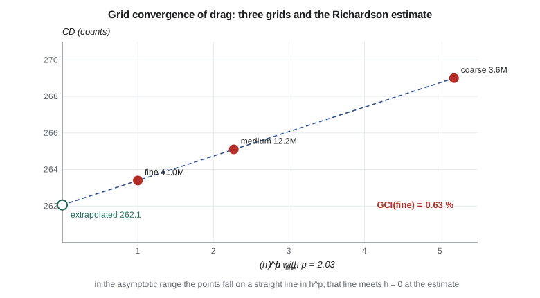
Solution verification estimates the numerical error of a particular calculation, where the exact answer is unknown. Iterative error is controlled by converging residuals and forces, as in lesson 5. Discretization error is estimated by solving on a sequence of systematically refined grids. If the grids are fine enough that the leading error term dominates, the asymptotic range, a quantity \(f\) computed on a grid with spacing \(h\) behaves as \(f_h = f_{\text{exact}} + C h^{p}\). Three grids give three equations for the three unknowns \(f_{\text{exact}}\), \(C\) and \(p\). With a constant refinement ratio \(r = h_2/h_1\), the observed order and the Richardson extrapolation are
where 1 is the finest grid. Patrick Roache proposed reporting the result as a grid convergence index, GCI, which converts the Richardson error estimate into an uncertainty band with a factor of safety \(F_s\), 1.25 when three grids show consistent behavior:
For three-dimensional unstructured grids, the representative spacing is \(h = (V/N)^{1/3}\), so the refinement ratio follows from the cell counts. The grids must be refined systematically, keeping the same topology and the same relative distribution of cells, including the first-cell height in wall units. Refining only the far field, or only the surface, does not give an order. The Tern Block 2 grids from lesson 6 have 3.6, 12.2 and 41.0 million cells, a refinement ratio of about 1.5 in each direction. The tunnel comparison runs at the tunnel Reynolds number of about 1.2 million, so the drag is higher than the flight value in lesson 8, because skin friction is higher at lower Reynolds number.
# Solution verification by Richardson extrapolation and the grid convergence index (GCI, Roache),
# then a validation comparison in the style of ASME V&V 20. Values are for the Tern Block 2 at the tunnel test condition.
import math
def gci(N, f, Fs=1.25, dim=3):
    (N1, N2, N3), (f1, f2, f3) = N, f                   # 1 = finest grid
    r21 = (N1 / N2) ** (1 / dim); r32 = (N2 / N3) ** (1 / dim)
    e21, e32 = f2 - f1, f3 - f2
    s = 1 if e32 / e21 > 0 else -1
    p = 1.0
    for _ in range(100):                                # fixed-point iteration for unequal ratios
        q = math.log((r21**p - s) / (r32**p - s))
        p = abs(math.log(abs(e32 / e21)) + q) / math.log(r21)
    f_ext = (r21**p * f1 - f2) / (r21**p - 1)
    g = Fs * abs(e21 / f1) / (r21**p - 1)
    return r21, r32, p, f_ext, g, s
N = (41.0e6, 12.2e6, 3.6e6)
res = {}
for name, f in (("drag coefficient (counts)", (263.4, 265.1, 269.0)), ("lift coefficient", (0.4512, 0.4498, 0.4461))):
    r21, r32, p, fx, g, s = gci(N, f); res[name] = g
    print(f"{name}: grids {N[0]/1e6:.1f}M / {N[1]/1e6:.1f}M / {N[2]/1e6:.1f}M cells")
    print(f"  refinement ratios r21 = {r21:.3f}, r32 = {r32:.3f}; {'monotone' if s > 0 else 'oscillatory'} convergence")
    print(f"  observed order p = {p:.2f}; extrapolated value {fx:.4f}; GCI(fine) = {100 * g:.2f} %")
print()
# Validation: E = S - D, with u_val combining numerical, input and experimental uncertainties
S, D = 263.4, 259.0                         # simulation and wind-tunnel drag (counts), corrected tunnel data
u_num = res["drag coefficient (counts)"] * S / 2   # GCI read as a band of about two standard uncertainties
u_in, u_D = 1.6, 2.5                        # from inflow and geometry sensitivities; tunnel balance and corrections
u_val = math.sqrt(u_num**2 + u_in**2 + u_D**2)
E = S - D
print(f"Comparison error E = S - D = {E:+.1f} counts")
print(f"  u_num = {u_num:.2f}, u_input = {u_in:.2f}, u_D = {u_D:.2f}  ->  u_val = {u_val:.2f} counts")
lo, hi = E - 2 * u_val, E + 2 * u_val
print(f"  model error lies in E +/- 2 u_val = {lo:+.1f} to {hi:+.1f} counts: " +
("the interval includes zero, so no model error is resolved" if lo < 0 < hi else "a model error is resolved"))drag coefficient (counts): grids 41.0M / 12.2M / 3.6M cells refinement ratios r21 = 1.498, r32 = 1.502; monotone convergence observed order p = 2.03; extrapolated value 262.0626; GCI(fine) = 0.63 % lift coefficient: grids 41.0M / 12.2M / 3.6M cells refinement ratios r21 = 1.498, r32 = 1.502; monotone convergence observed order p = 2.38; extrapolated value 0.4521; GCI(fine) = 0.24 % Comparison error E = S - D = +4.4 counts u_num = 0.84, u_input = 1.60, u_D = 2.50 -> u_val = 3.08 counts model error lies in E +/- 2 u_val = -1.8 to +10.6 counts: the interval includes zero, so no model error is resolved
Drag converges monotonically, falling from 269.0 to 265.1 to 263.4 counts, with an observed order of 2.03, close to the scheme's formal second order. That agreement is the best evidence that the grids are in the asymptotic range. The extrapolated drag is 262.1 counts and the GCI on the finest grid is 0.63 percent, about 1.7 counts. Lift also converges monotonically, with an observed order of 2.38 and a GCI of 0.24 percent. An observed order far from the formal order, or oscillatory convergence, is a warning: the grids may not be in the asymptotic range, limiters may be active, or the grids may not be similar. In such cases a larger factor of safety, 3.0, is recommended, or more grids are needed.
Validation
Validation compares the simulation result \(S\) with an experimental value \(D\) for the same quantity under the same conditions. ASME V&V 20 defines the comparison error \(E = S - D\) and a validation uncertainty that combines the numerical uncertainty, the uncertainty in the simulation inputs and the uncertainty in the experimental data:
The model-form error, the quantity validation seeks, then lies within \(E \pm k\,u_{\text{val}}\), where \(k\) sets the confidence level. If \(|E|\) is much larger than \(u_{\text{val}}\), a model error of about \(E\) is indicated. If \(|E|\) is comparable to or smaller than \(u_{\text{val}}\), the model error cannot be distinguished from the noise of the comparison. For the Tern Block 2, the simulation gives 263.4 counts and the corrected tunnel drag is 259.0 counts, so \(E = +4.4\) counts. The input uncertainty, 1.6 counts, comes from running the solver at the extremes of the tunnel's Mach number and angle-of-attack uncertainty and with the as-measured model geometry. The tunnel uncertainty, 2.5 counts, combines balance accuracy, repeatability and the uncertainty of the wall and support corrections. With \(u_{\text{val}} = 3.1\) counts and \(k = 2\), the model error lies between about \(-1.8\) and \(+10.6\) counts. The comparison does not resolve a model error, but it bounds it.
That bound is useful. It tells the program that, at this condition, RANS with the Spalart-Allmaras model predicts drag to within about 11 counts of the tunnel, and that the numerical error is the smallest contributor. To tighten the bound, the experiment's uncertainty would have to fall, not the grid's. Such conclusions are only possible because each uncertainty was estimated separately.
| Source | Standard uncertainty (counts) | How it was estimated |
|---|---|---|
| Numerical, \(u_{\text{num}}\) | 0.84 | GCI on the fine grid, read as about two standard uncertainties |
| Simulation inputs, \(u_{\text{input}}\) | 1.6 | Runs at the extremes of tunnel Mach number, angle and geometry uncertainty |
| Experiment, \(u_D\) | 2.5 | Balance accuracy, repeatability, wall and support corrections |
| Validation, \(u_{\text{val}}\) | 3.1 | Root-sum-square of the three |
Lessons from the workshops
The AIAA Drag Prediction Workshops, which began in 2001, invited groups worldwide to compute the same transport configurations on common and their own grids, with experimental data for comparison. Their findings have shaped industrial practice. The spread between participants' drag predictions was, in the early workshops, several tens of counts, far larger than the few counts that matter commercially. Much of the spread came from grids and user practice, and it narrowed as gridding guidelines and grid families improved. Results using the same turbulence model clustered more tightly than results using different models. Predictions of increments, such as the drag change from adding a nacelle, were more consistent than absolute values. The High Lift Prediction Workshops found larger scatter near maximum lift, where separation dominates. These lessons appear in the group's practice: common grid families, a default turbulence model named exactly, and an emphasis on increments.
Credibility and reporting
A CFD report that will support a decision must let the reader judge its credibility. The group's reports state the intended use, the code and version, the turbulence model variant, the grids and their quality, the convergence criteria, the grid study with observed order and GCI, the validation evidence for similar flows and its uncertainty, and the known limitations. For certification, the FAA expects analysis methods to be validated for the conditions where they are used, generally through comparison with test data from similar configurations, and Rachel's plan uses CFD to support, rather than replace, the tunnel and flight tests that demonstrate compliance.
Worked problem
Observed order from three grids
Lift on three grids with \(r = 1.5\) is 0.4461, 0.4498 and 0.4512 from coarse to fine. Find the observed order.
Show solution
- \(f_3 - f_2 = 0.4461 - 0.4498 = -0.0037\), with 1 the finest grid.
- \(f_2 - f_1 = 0.4498 - 0.4512 = -0.0014\). Both differences have the same sign, so convergence is monotone.
- \(p = \ln(0.0037/0.0014)/\ln 1.5 = \ln 2.643/0.4055 = 2.40\).
Answer: About 2.4, consistent with the code's 2.38 (which uses the exact refinement ratios).
Worked problem
Richardson extrapolation for drag
With fine and medium drag of 263.4 and 265.1 counts, \(r = 1.5\) and \(p = 2.03\), find the extrapolated drag.
Show solution
- \(r^{p} = 1.5^{2.03} = 2.278\).
- \(f_{\text{ext}} = (2.278 \times 263.4 - 265.1)/(2.278 - 1)\).
- \(= (600.0 - 265.1)/1.278 = 262.1\).
Answer: 262.1 counts, 1.3 counts below the fine-grid value.
Worked problem
Is a model error resolved?
At a higher lift coefficient, the simulation gives 312 counts, the tunnel 296 counts, and \(u_{\text{val}} = 4.0\) counts. What can be concluded with \(k = 2\)?
Show solution
- \(E = 312 - 296 = 16\) counts.
- Interval: \(16 \pm 8\), from 8 to 24 counts.
- The interval excludes zero.
Answer: A model error of 8 to 24 counts is resolved: the simulation overpredicts drag at this condition, likely from separation near the trailing edge that the model overestimates.
Common mistakes
MistakeVerification and validation mean the same thing.
InsteadVerification checks that equations are solved correctly; validation checks that they are the right equations for the purpose.
MistakeAgreement with one experiment validates a code.
InsteadValidation applies to a specific use and range of conditions, and requires uncertainty estimates for both simulation and experiment.
MistakeAny three grids give a valid GCI.
InsteadThe grids must be systematically refined and in the asymptotic range; erratic orders call for more grids or a larger factor of safety.
MistakeIf simulation and test disagree, the simulation is wrong.
InsteadExperimental data have uncertainties and corrections too; the comparison must account for both.
Summary and key terms
- Verification checks that the equations are solved correctly; validation checks that the model represents reality for an intended use.
- Code verification uses manufactured and exact solutions to confirm the order of accuracy.
- Solution verification uses systematically refined grids, Richardson extrapolation and the grid convergence index to estimate discretization error.
- Validation, as in ASME V&V 20, compares the comparison error with a validation uncertainty built from numerical, input and experimental uncertainties.
- Workshop experience shows the importance of common grids, exact model naming and increments.
- Verification
- Determining that a model is solved correctly.
- Validation
- Determining how well a model represents reality for an intended use.
- Method of manufactured solutions
- Code verification using an assumed exact solution and the source terms it requires.
- Richardson extrapolation
- Estimating the zero-spacing value from solutions on refined grids.
- Grid convergence index
- An uncertainty estimate for discretization error based on Richardson extrapolation and a factor of safety.
- Comparison error
- The difference between simulation and experimental values.
- Validation uncertainty
- The combined uncertainty of numerical, input and experimental contributions.
Practice problems
Work each problem on paper first, then reveal the answer to check.
What factor of safety is recommended for the GCI with three grids in the asymptotic range?
Show answer
1.25.
What is the refinement ratio between grids of 12.2 and 41.0 million cells?
Show answer
\((41.0/12.2)^{1/3} = 1.498\).
Why are increments more reliable than absolute values?
Show answer
Many errors are similar between two nearby configurations and cancel in the difference.
What does it mean if the observed order is 0.6 for a second-order scheme?
Show answer
The grids are probably not in the asymptotic range, or something such as limiter activity or grid dissimilarity is affecting convergence.
Name the three components of the validation uncertainty.
Show answer
Numerical, input and experimental.
Lesson quiz · 5 questions
Score 60% or more to complete this lesson.
Create a free account to save your progress, take quizzes and earn a certificate.