
AERO-440 · Lesson 8 of 12 · 24 min
Viscous flows and the Navier-Stokes equations
The Euler screen picked a section for the Swift 900, but the drag that matters to the airline customers is mostly viscous: on a business jet at cruise, skin friction and form drag together make up more than half of the total. The Petrel 19 is the same story at lower speed, with large wetted areas on its high wing, fuselage and nacelles. To predict that drag, the group must solve the Navier-Stokes equations, which add viscosity and heat conduction to the Euler equations. This lesson covers the equations, how their viscous terms are discretized, and a first validation: a laminar flat-plate boundary layer, for which an exact similarity solution exists.
The Navier-Stokes equations
The compressible Navier-Stokes equations keep the conservation form of the Euler equations and add a viscous flux. In compact form,
The convective flux \(\mathbf{F}_c\) is the Euler flux. The viscous flux \(\mathbf{F}_v\) contains the viscous stress tensor in the momentum equations and, in the energy equation, the work done by viscous stresses and the heat conducted. For a Newtonian fluid with Stokes' hypothesis, the stress tensor is
The dynamic viscosity \(\mu\) of air varies with temperature, usually through Sutherland's law, and the thermal conductivity \(k\) is linked to it through a Prandtl number of about 0.72. Making the equations dimensionless with a reference length, velocity and density brings out the governing parameters: the Reynolds number, the ratio of inertial to viscous forces, the Mach number and the Prandtl number. At the Tern Block 2 cruise condition, the Reynolds number based on mean chord is about \(10^{7}\): viscous effects are confined to thin layers next to the surfaces and in the wakes, but those layers decide the drag and, near stall, the lift.
The viscous terms change the mathematical character of the equations. The steady Navier-Stokes equations are no longer purely hyperbolic; the viscous terms are second derivatives, which are parabolic in time and elliptic in space. Every point in a viscous flow influences its neighbors by diffusion, and the boundary conditions change accordingly. At a solid wall, the no-slip condition sets all velocity components to zero, and a thermal condition fixes either the wall temperature or the heat flux; an adiabatic wall, with zero heat flux, is the usual choice for external aerodynamics.
Discretizing the viscous terms
In a finite-volume code, the viscous flux at each face needs the velocity and temperature gradients there. On a structured grid, these come from central differences across the face, which are second order and naturally stable because diffusion damps errors. On unstructured grids, the face gradient is usually built from the average of the two cell gradients, corrected with the direct difference between the two cell values along the line joining their centers. The correction matters: averaged gradients alone can let odd-even oscillations go undamped, and on stretched or skewed boundary-layer cells the uncorrected scheme loses accuracy. Viscous terms are central-differenced, never upwinded, because diffusion has no preferred direction.
The viscous terms also make the equations stiff. In a boundary-layer cell a few micrometers thick, the viscous time scale \(\Delta y^{2}/\nu\) is extremely short, as lesson 5 showed. Implicit treatment of at least the wall-normal viscous terms is therefore standard. The resolution requirement is equally severe: lesson 6 showed that \(y^{+} \approx 1\) at the wall means first cells of about 5 micrometers on the Tern Block 2, and the boundary layer needs perhaps 30 to 40 cells across its thickness to resolve the velocity profile.
A laminar check: the Blasius boundary layer
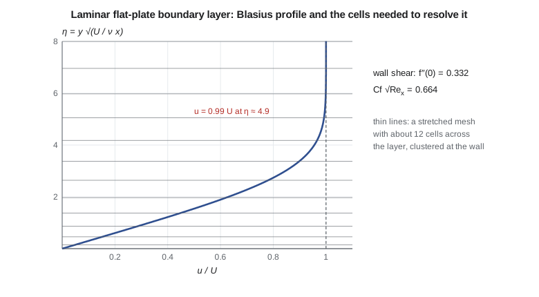
Before trusting a viscous solver with turbulence, the group checks it on laminar flow, where the physics is exact and only numerical error remains. The laminar boundary layer on a flat plate with zero pressure gradient has a similarity solution found by Heinrich Blasius in 1908. Introducing the similarity variable \(\eta = y\sqrt{U/(\nu x)}\) and a stream function \(\psi = \sqrt{\nu U x}\, f(\eta)\), the boundary-layer equations collapse to a single ordinary differential equation:
The velocity profile is \(u/U = f'(\eta)\). The wall shear stress follows from \(f''(0)\), which gives the local skin-friction coefficient \(C_f = 0.664/\sqrt{Re_x}\). The equation is solved by shooting: guess \(f''(0)\), integrate outward, and adjust the guess until \(f'\) approaches 1 far from the wall. The code below does this with a fourth-order Runge-Kutta integrator and bisection. It then solves the same flow a second way, by marching the boundary-layer equations downstream on a finite-difference grid, implicit across the layer with the Thomas algorithm from lesson 3 and with the normal velocity found from continuity. The marching solver is a simplified relative of a full Navier-Stokes code: it keeps the dominant viscous term and convection, and it must reproduce Blasius's answer.
# Laminar flat-plate boundary layer two ways:
# (1) Blasius similarity ODE f''' + 0.5 f f'' = 0 solved by shooting with RK4;
# (2) a marching finite-difference solution of the boundary-layer form of the Navier-Stokes equations,
#     implicit in y (Thomas algorithm), with v from continuity. Units: U = 1, nu = 1, so Re_x = x.
import math
def blasius(s, eta_max=10.0, n=2000):
    h = eta_max / n; y = [0.0, 0.0, s]
    def F(y): return [y[1], y[2], -0.5 * y[0] * y[2]]
    for _ in range(n):
        k1 = F(y); k2 = F([y[i] + h/2*k1[i] for i in range(3)])
        k3 = F([y[i] + h/2*k2[i] for i in range(3)]); k4 = F([y[i] + h*k3[i] for i in range(3)])
        y = [y[i] + h/6*(k1[i] + 2*k2[i] + 2*k3[i] + k4[i]) for i in range(3)]
    return y[1] - 1.0                                  # want f'(inf) = 1
a, b = 0.2, 0.5
for _ in range(60):                                    # bisection on f''(0)
    m = 0.5 * (a + b)
    if blasius(a) * blasius(m) <= 0: b = m
    else: a = m
fpp = 0.5 * (a + b)
print(f"Blasius f''(0) = {fpp:.5f}  ->  Cf * sqrt(Re_x) = {2 * fpp:.4f}")
def thomas(lo, di, up, rhs):
    n = len(di); c = [0.0] * n; d = [0.0] * n
    c[0] = up[0] / di[0]; d[0] = rhs[0] / di[0]
    for i in range(1, n):
        den = di[i] - lo[i] * c[i - 1]
        c[i] = up[i] / den if i < n - 1 else 0.0
        d[i] = (rhs[i] - lo[i] * d[i - 1]) / den
    x = [0.0] * n; x[-1] = d[-1]
    for i in range(n - 2, -1, -1): x[i] = d[i] - c[i] * x[i + 1]
    return x
def march(ny, x_end=1.0, nx=400):
    Y = 12.0 * math.sqrt(x_end); dy = Y / ny
    u = [1.0] * (ny + 1); u[0] = 0.0; v = [0.0] * (ny + 1)
    x = 1e-4
    for k in range(nx):
        x_new = 1e-4 + (x_end - 1e-4) * ((k + 1) / nx) ** 2    # finer steps near the leading edge
        dx = x_new - x
        lo = [0.0]; di = [1.0]; up = [0.0]; rhs = [0.0]        # wall: u = 0
        for j in range(1, ny):
            uj = max(u[j], 1e-6)
            lo.append(-v[j] / (2 * dy) - 1 / dy**2)
            di.append(uj / dx + 2 / dy**2)
            up.append(v[j] / (2 * dy) - 1 / dy**2)
            rhs.append(uj * u[j] / dx)
        lo.append(0.0); di.append(1.0); up.append(0.0); rhs.append(1.0)   # edge: u = 1
        un = thomas(lo, di, up, rhs)
        vn = [0.0] * (ny + 1)
        for j in range(1, ny + 1):                              # continuity, trapezoidal in y
            dudx = 0.5 * ((un[j] - u[j]) + (un[j - 1] - u[j - 1])) / dx
            vn[j] = vn[j - 1] - dudx * dy
        u, v, x = un, vn, x_new
    tau = (-3 * u[0] + 4 * u[1] - u[2]) / (2 * dy)              # second-order wall gradient
    return 2 * tau * math.sqrt(x)                               # Cf * sqrt(Re_x)
print("Marching solution at Re_x = 1 (similarity makes the result independent of Re_x):")
prev = None
for ny, nx in ((25, 100), (50, 200), (100, 400), (200, 800)):
    val = march(ny, nx=nx)
    err = abs(val - 2 * fpp)
    print(f"  {ny:3d} x {nx:3d} grid: Cf*sqrt(Re_x) = {val:.4f}, error {err:.4f}" +
          ("" if prev is None else f", ratio {prev / err:.2f}"))
prev = errBlasius f''(0) = 0.33206 -> Cf * sqrt(Re_x) = 0.6641 Marching solution at Re_x = 1 (similarity makes the result independent of Re_x): 25 x 100 grid: Cf*sqrt(Re_x) = 0.6585, error 0.0056 50 x 200 grid: Cf*sqrt(Re_x) = 0.6586, error 0.0056, ratio 1.01 100 x 400 grid: Cf*sqrt(Re_x) = 0.6612, error 0.0029, ratio 1.89 200 x 800 grid: Cf*sqrt(Re_x) = 0.6627, error 0.0014, ratio 2.13
Shooting gives \(f''(0) = 0.33206\) and \(C_f\sqrt{Re_x} = 0.6641\), the classical values. The marching solver approaches this result as both the wall-normal and the streamwise grids are refined, reaching 0.6627 on the finest grid. On the two finest grids the error halves with each refinement, the signature of first-order accuracy in the marching direction, since the scheme uses a backward step in \(x\). On the two coarsest grids the error barely changes, because two errors of opposite sign, from the coarse wall-normal grid and from the start at the leading edge, partly cancel. This is a lesson in itself: an error that does not change between two grids does not prove the solution is converged. Only a systematic study across three or more grids, lesson 10, shows whether the results lie in the asymptotic range.
Separation and the pressure gradient
The flat plate has no pressure gradient. On a wing, the pressure falls from the stagnation point to the suction peak and then rises toward the trailing edge. An adverse pressure gradient, rising pressure in the flow direction, decelerates the slow fluid near the wall, and if it is strong enough, the near-wall flow reverses and the boundary layer separates. Separation is where the Navier-Stokes equations show their value and where they make the greatest demands. A separated region is thick, often unsteady, and highly sensitive to the state of the boundary layer upstream, laminar or turbulent. Predicting separation on the Tern Block 2 wing near stall and on the Petrel 19 nacelle afterbody is the central difficulty of the next two lessons.
Laminar, transitional and turbulent flow
At flight Reynolds numbers, boundary layers on aircraft are mostly turbulent. On the Tern Block 2 wing, the boundary layer begins laminar at the leading edge and undergoes transition, usually within the first 10 to 40 percent of chord depending on the pressure distribution and surface finish. Direct solution of the Navier-Stokes equations, DNS, would resolve the turbulent eddies, but lesson 1 showed that DNS of a wing at flight Reynolds number is out of reach. RANS solvers average the equations in time, so that the eddies are represented by a turbulence model. The averaged equations look like the Navier-Stokes equations with an extra stress, the Reynolds stress, and closing them is the subject of lesson 9.
| Viscous drag contribution, Tern Block 2 at cruise (RANS, medium grid) | Counts |
|---|---|
| Wing skin friction | 58 |
| Fuselage skin friction | 41 |
| Pressure (form) drag, wing and fuselage | 19 |
| Induced drag | 96 |
| Interference and other | 12 |
| Total, wing-body | 226 |
The breakdown shows why a viscous solver is indispensable. Skin friction and form drag together make up more than half of the wing-body drag at cruise, and none of them appears in an Euler solution. It also shows where RANS is strong. Skin friction on attached, turbulent surfaces is predicted to within a few percent by good turbulence models on adequate grids, provided the transition location is right. Form drag and interference drag are harder, because they depend on the pressure recovery near trailing edges and junctions, where separation can begin.
Worked problem
Blasius skin friction and drag
Estimate the laminar skin-friction drag on one side of a flat plate 0.5 m long and 1 m wide in air at 30 m/s, with \(\nu = 1.5 \times 10^{-5}\ \mathrm{m^2/s}\) and \(\rho = 1.2\ \mathrm{kg/m^3}\).
Show solution
- \(Re_L = 30 \times 0.5/1.5 \times 10^{-5} = 10^{6}\), at the upper edge of the laminar range.
- Average skin friction for Blasius: \(\bar{C}_f = 1.328/\sqrt{Re_L} = 0.00133\).
- \(D = \tfrac12\rho V^{2} S \bar{C}_f = 0.5 \times 1.2 \times 900 \times 0.5 \times 0.00133 = 0.36\ \mathrm{N}\).
Answer: About 0.36 N. A turbulent layer at the same Reynolds number would give roughly three times as much.
Worked problem
Boundary-layer thickness
How thick is the laminar layer at the end of that plate, using \(\delta_{99} \approx 4.9\,x/\sqrt{Re_x}\)?
Show solution
- \(\sqrt{Re_x} = 1000\).
- \(\delta_{99} = 4.9 \times 0.5/1000 = 2.45\ \mathrm{mm}\).
Answer: About 2.5 mm, so a grid needs cells of a fraction of a millimeter across it to resolve the profile.
Worked problem
Reading a convergence table
The code reports errors of 0.0056 on the two coarsest grids and 0.0029 and 0.0014 on the next two. Arjun says the coarse result proves the solution was converged. Is he right?
Show solution
- An unchanged error between two grids can come from canceling errors, not from convergence.
- The finer grids show the error halving, so the result was not converged on the coarse grids.
- Asymptotic behavior must be shown on at least three grids.
Answer: No. The coarse grids lie outside the asymptotic range, and the agreement between them is a coincidence of canceling errors.
Common mistakes
MistakeThe no-slip condition only affects the first cell.
InsteadIt controls the whole boundary layer, and the first cell must be thin enough to resolve the near-wall gradient.
MistakeViscous terms should be upwinded like convective ones.
InsteadDiffusion has no preferred direction; viscous terms are central-differenced.
MistakeTwo grids that give the same answer prove grid independence.
InsteadCanceling errors can make two coarse grids agree; use three or more grids and check the observed order.
MistakeEuler drag plus a flat-plate friction estimate gives total drag.
InsteadForm and interference drag depend on the coupled viscous flow, especially near trailing edges and junctions.
Summary and key terms
- The Navier-Stokes equations add a viscous stress and heat flux to the Euler equations, with the Reynolds, Mach and Prandtl numbers as governing parameters.
- Viscous terms are central-differenced and usually treated implicitly because they are stiff on thin wall cells.
- The no-slip condition and an adiabatic or isothermal wall condition replace the inviscid slip condition.
- The Blasius solution, with \(C_f\sqrt{Re_x} = 0.664\), is a standard check of a viscous solver, and a systematic grid study is needed to show convergence.
- Viscous drag makes up much of an aircraft's total, and separation in adverse pressure gradients is where viscous prediction is hardest.
- Navier-Stokes equations
- The conservation laws for a viscous, heat-conducting fluid.
- No-slip condition
- Zero fluid velocity relative to a solid wall.
- Sutherland law
- A formula for the temperature dependence of the viscosity of a gas.
- Blasius solution
- The similarity solution for the laminar boundary layer on a flat plate.
- Adverse pressure gradient
- Pressure rising in the flow direction, which decelerates the boundary layer.
- Separation
- Breakaway of the boundary layer from the surface, with reversed flow near the wall.
- Drag count
- One ten-thousandth of a drag coefficient.
Practice problems
Work each problem on paper first, then reveal the answer to check.
What is \(C_f\) for a laminar boundary layer at \(Re_x = 4 \times 10^{5}\)?
Show answer
\(0.664/632 = 0.00105\).
Why is an adiabatic wall the usual thermal condition for external aerodynamics?
Show answer
Heat transfer to and from the skin is small at subsonic speeds, so zero heat flux is a good approximation.
What does Stokes' hypothesis set?
Show answer
The bulk viscosity to zero, giving the factor \(-2/3\) in the stress tensor.
Which drag components does an Euler solver omit?
Show answer
Skin friction and viscous form drag.
What is the order of accuracy of the marching solver in the streamwise direction?
Show answer
First order, since it uses a backward difference in \(x\).
Lesson quiz · 5 questions
Score 60% or more to complete this lesson.
Create a free account to save your progress, take quizzes and earn a certificate.