
STAT-151 · Lesson 3 of 12 · 32 min
Probability and Bayes’ theorem
Probability is the language statistics uses to describe uncertainty. When we say a new antibiotic cures 80 per cent of infections, that a seed has a 0.6 chance of germinating, or that a test result has a 5 per cent chance of being a false alarm, we are making probability statements. This lesson sets out the rules of probability that the rest of the course relies on, with an emphasis on conditional probability and Bayes’ theorem, which are essential for interpreting diagnostic tests, screening programs and much of modern data analysis. The formal, axiomatic treatment of probability, including continuous distributions in depth, is the subject of STAT-251.
What probability means
There are two main interpretations of probability. The frequentist interpretation defines the probability of an event as its long-run relative frequency in many repetitions of the same process: if we toss a fair coin many times, the proportion of heads approaches 0.5. The Bayesian interpretation treats probability as a degree of belief, which can be updated as evidence accumulates; it can be applied to one-off events, such as the probability that a particular hypothesis is true. Most of this course uses frequentist methods, which dominate the scientific literature, but Bayes’ theorem itself is a rule of probability that both schools accept.
import numpy as np
rng = np.random.default_rng(151)

# Long-run relative frequency: germination of seeds with true probability 0.6
germinated = rng.random(10_000) < 0.6
for n in (10, 100, 1_000, 10_000):
print(f"after {n:6,d} seeds: proportion germinated = {germinated[:n].mean():.3f}")after 10 seeds: proportion germinated = 0.700 after 100 seeds: proportion germinated = 0.610 after 1,000 seeds: proportion germinated = 0.586 after 10,000 seeds: proportion germinated = 0.595
After ten seeds the proportion can be far from 0.6, but it settles toward 0.6 as the number of seeds grows. This tendency, called the law of large numbers, is what connects probabilities to observed data. The proportion approaches 0.6 only gradually; the size of the typical deviation shrinks with the square root of the number of trials, the same √n that appeared in the standard error in lesson 1.
Sample spaces, events and the basic rules
The sample space, S, is the set of all possible outcomes of a random process. An event is a set of outcomes. For a seed planted in a pot, the sample space might be {germinates and survives, germinates and dies, fails to germinate}, and the event ‘germinates’ contains the first two outcomes. Probabilities satisfy a few basic rules.
| Rule | Statement | Example |
|---|---|---|
| Range | 0 ≤ P(A) ≤ 1 | No probability is negative or above 1 |
| Total | P(S) = 1 | Some outcome must occur |
| Complement | P(not A) = 1 − P(A) | If P(germinate) = 0.6, P(fail) = 0.4 |
| Addition (general) | P(A or B) = P(A) + P(B) − P(A and B) | Subtract the overlap so it is not counted twice |
| Addition (disjoint) | P(A or B) = P(A) + P(B) if A and B cannot both occur | Blood types A and B in one person |
| Multiplication (general) | P(A and B) = P(A) × P(B | A) | Chain of conditional probabilities |
| Multiplication (independent) | P(A and B) = P(A) × P(B) | Two seeds germinating separately |
Two events are disjoint (mutually exclusive) if they cannot happen together. Two events are independent if knowing that one occurred does not change the probability of the other. These are very different ideas, and confusing them is a common error: disjoint events with positive probabilities are never independent, because knowing that one happened tells you the other did not.
Worked problem
At least one germinates
Each of five seeds germinates independently with probability 0.6. What is the probability that at least one germinates?
Show solution
- The complement of ‘at least one germinates’ is ‘none germinate’.
- P(none) = 0.4⁵ = 0.01024, using the multiplication rule for independent events.
- P(at least one) = 1 − 0.01024 = 0.98976.
Answer: About 0.990. Using the complement avoids adding up the probabilities of one, two, three, four and five germinating.
Conditional probability
The conditional probability of A given B, written P(A | B), is the probability that A occurs when we already know B has occurred. It is defined as the probability that both occur divided by the probability of B. Conditional probability restricts attention to the part of the sample space where B is true.
Two-way tables of counts make conditional probabilities concrete. The table below gives invented results from a survey of 1,000 trees for a fungal disease, classified by whether each tree was near a road where de-icing salt was used.
| Diseased | Healthy | Total | |
|---|---|---|---|
| Near road | 90 | 210 | 300 |
| Away from road | 70 | 630 | 700 |
| Total | 160 | 840 | 1,000 |
Overall, P(diseased) = 160/1,000 = 0.16. Among trees near roads, P(diseased | near road) = 90/300 = 0.30; among trees away from roads, P(diseased | away) = 70/700 = 0.10. Disease and location are not independent, because the conditional probability of disease depends on location. Whether the salt causes the disease is a separate question; this is an observational survey, so confounders such as soil compaction or tree age could be responsible (lesson 1). Lesson 9 shows how to test whether such an association could be due to chance.
It is crucial to distinguish P(A | B) from P(B | A). Here, P(near road | diseased) = 90/160 = 0.56, which is quite different from P(diseased | near road) = 0.30. Swapping the two, sometimes called the prosecutor’s fallacy when it occurs in court, is one of the most consequential errors in reasoning about evidence.
Independence and its failures
Many calculations multiply probabilities on the assumption of independence, and this assumption deserves suspicion. Seeds in the same pot share soil and water, so their germination is not independent. Patients in the same hospital ward share exposures. Cases in an infectious disease outbreak are dependent by definition. The pseudoreplication problem of lesson 1 is, at heart, a failure of independence: measurements from the same tank are positively correlated, so treating them as independent overstates the information they contain.
Bayes’ theorem
Bayes’ theorem reverses a conditional probability. It expresses P(A | B) in terms of P(B | A) and the overall probability of A. Combined with the law of total probability, which computes P(B) by adding up the ways B can occur, it gives a formula that is used every day in medicine, ecology and machine learning.
In Bayesian language, P(A) is the prior probability of A before seeing the evidence, P(B | A) is the likelihood of the evidence if A is true, and P(A | B) is the posterior probability after seeing the evidence. The formula shows that the posterior depends strongly on the prior: strong evidence for a rare event may still leave it fairly unlikely.
Diagnostic tests: sensitivity, specificity and predictive values
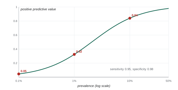
Diagnostic and screening tests are the most important everyday application of Bayes’ theorem. A test’s sensitivity is the probability it is positive when the condition is present, P(+ | disease). Its specificity is the probability it is negative when the condition is absent, P(− | no disease). These are properties of the test, measured in validation studies. But a patient or clinician wants the reverse: given a positive result, how likely is disease? That is the positive predictive value (PPV), P(disease | +). The negative predictive value (NPV) is P(no disease | −). Predictive values depend on the prevalence of the condition in the population being tested, which plays the role of the prior.
Worked problem
A screening test for a rare condition
A screening test has sensitivity 0.95 and specificity 0.98. The condition affects 1 in 500 people in the population screened. What is the probability that a person who tests positive has the condition?
Show solution
- Prior: P(D) = 1/500 = 0.002, so P(not D) = 0.998.
- P(+ | D) = 0.95; P(+ | not D) = 1 − 0.98 = 0.02.
- P(+) = 0.95 × 0.002 + 0.02 × 0.998 = 0.0019 + 0.01996 = 0.02186.
- PPV = 0.0019 / 0.02186 ≈ 0.087.
Answer: Only about 9 per cent of positives have the condition: false positives from the large healthy population outnumber true positives about ten to one.
The result surprises many people, including many health professionals in survey studies. A useful way to see it is with natural frequencies: of 100,000 people screened, 200 have the condition and about 190 of them test positive, while 99,800 do not and about 1,996 of them test positive anyway. Of the 2,186 positives, only 190 are true positives. This is why screening programs for rare conditions use a positive screen as a reason for a more specific confirmatory test, not as a diagnosis.
def predictive_values(sens, spec, prev):
    tp = sens * prev
    fp = (1 - spec) * (1 - prev)
    fn = (1 - sens) * prev
    tn = spec * (1 - prev)
    return tp / (tp + fp), tn / (tn + fn)

sens, spec = 0.95, 0.98
print("prevalence    PPV     NPV")
for prev in (0.001, 0.002, 0.01, 0.05, 0.20, 0.50):
    ppv, npv = predictive_values(sens, spec, prev)
print(f"{prev:9.3f} {ppv:6.3f} {npv:7.4f}")prevalence PPV NPV
0.001 0.045 0.9999
0.002 0.087 0.9999
0.010 0.324 0.9995
0.050 0.714 0.9973
0.200 0.922 0.9874
0.500 0.979 0.9515The same test that is nearly useless as a stand-alone diagnosis in general screening becomes highly informative when used on patients with symptoms, among whom the condition is common. At a prevalence of 20 per cent, a positive result means the condition is very likely. This dependence on prevalence explains why guidelines from bodies such as the Public Health Agency of Canada and the US Centers for Disease Control and Prevention recommend different testing strategies for people with and without symptoms or known exposures.
Sequential testing and updating
Bayes’ theorem can be applied repeatedly. The posterior from one test becomes the prior for the next, provided the tests make errors independently given the true condition. If the person in the screening example who tested positive (posterior 0.087) takes a second, independent test with the same accuracy and is positive again, the new posterior is about 0.82. Two positives from independent tests are far more convincing than one. In practice, the second test is usually a different, more specific method, because repeating the same test can repeat the same error, for example when a cross-reacting substance in the person’s blood causes the false positive.
def update(prior, sens, spec, positive=True):
    if positive:
        num = sens * prior; den = num + (1 - spec) * (1 - prior)
    else:
        num = (1 - sens) * prior; den = num + spec * (1 - prior)
    return num / den

p = 0.002
for i, result in enumerate([True, True], 1):
    p = update(p, 0.95, 0.98, result)
print(f"after test {i} ({'positive' if result else 'negative'}): P(condition) = {p:.3f}")after test 1 (positive): P(condition) = 0.087 after test 2 (positive): P(condition) = 0.819
Bayes’ theorem in ecology and genetics
Bayesian reasoning appears throughout science. In wildlife surveys, a species may be present at a site but missed by the observer; occupancy models use the detection probability, measured from repeat visits, to estimate the probability that a site is truly occupied given that the species was not seen. In genetics, a genetic counsellor uses Bayes’ theorem to update the probability that a woman is a carrier of an X-linked condition after she has had several unaffected sons, as BIOL-201 shows. In each case the logic is the same: combine what was known beforehand with how likely the observed evidence is under each possibility.
Worked problem
Was the frog really absent?
A rare frog occupies about 30 per cent of suitable ponds in a region. A single night survey detects the frog at an occupied pond with probability 0.6. A survey finds no frogs. What is the probability that the pond is nevertheless occupied?
Show solution
- Prior P(occupied) = 0.3; P(not detected | occupied) = 0.4; P(not detected | unoccupied) = 1.
- P(not detected) = 0.4 × 0.3 + 1 × 0.7 = 0.82.
- P(occupied | not detected) = 0.12 / 0.82 ≈ 0.146.
- After a second survey that also finds nothing: P(not detected twice | occupied) = 0.16, so the posterior is 0.048 / (0.048 + 0.7) ≈ 0.064.
Answer: About 15 per cent after one negative survey and about 6 per cent after two; a single negative survey is weak evidence of absence.
Counting and probabilities of combinations
When all outcomes are equally likely, probabilities can be found by counting. The number of ways to choose k items from n, ignoring order, is the binomial coefficient, written C(n, k) or n choose k, equal to n!/(k!(n − k)!). It counts, for example, how many ways 3 of 10 seedlings could be the ones that die. Binomial coefficients reappear in lesson 4 in the binomial distribution, and they underlie Fisher’s exact test in lesson 9. CMPUT-272 develops counting methods in more depth.
from math import comb
# Probability that the 3 seedlings that died all came from the 5 in the treated group,
# if deaths were spread at random among 10 seedlings (5 treated, 5 control)
ways_all_treated = comb(5, 3)
ways_total = comb(10, 3)
print(f"C(5,3) = {ways_all_treated}, C(10,3) = {ways_total}, probability = {ways_all_treated/ways_total:.3f}")C(5,3) = 10, C(10,3) = 120, probability = 0.083
If deaths were unrelated to treatment, all three deaths would fall in the treated group about 8 per cent of the time. That is unusual but not rare enough to be convincing; this kind of reasoning, comparing an observed outcome with how often chance alone would produce it, is the foundation of the hypothesis tests in lesson 7.
Common mistakes
MistakeP(A | B) and P(B | A) are interchangeable.
InsteadThey are usually very different; Bayes’ theorem is needed to convert one into the other.
MistakeDisjoint events are independent.
InsteadDisjoint events with positive probabilities are dependent: if one occurs, the other cannot.
MistakeA test with 95 per cent sensitivity means a positive result is 95 per cent likely to be correct.
InsteadThe probability a positive is correct (PPV) depends on prevalence and specificity and can be much lower.
MistakeProbabilities of separate events can always be multiplied.
InsteadMultiplication without conditional probabilities requires independence, which often fails for clustered or shared exposures.
MistakeA species not found in a survey is absent.
InsteadImperfect detection means non-detection is only partial evidence of absence; Bayes’ theorem quantifies how much.
Summary and key terms
- Probability can be read as long-run relative frequency or as a degree of belief; the law of large numbers links probability to observed proportions.
- The complement, addition and multiplication rules allow probabilities of combined events to be calculated.
- Conditional probability restricts attention to cases where a given event occurred; P(A | B) and P(B | A) generally differ.
- Independence means one event does not change the probability of another; it often fails for clustered data.
- Bayes’ theorem combines a prior probability with the likelihood of evidence to give a posterior probability.
- Sensitivity and specificity describe a test; predictive values describe what a result means and depend strongly on prevalence.
- Sequential independent evidence can be combined by using each posterior as the next prior.
- sample space
- The set of all possible outcomes of a random process.
- independent events
- Events for which the occurrence of one does not change the probability of the other.
- conditional probability
- The probability of an event given that another event has occurred.
- Bayes’ theorem
- A rule for reversing conditional probabilities, combining a prior with the likelihood of evidence.
- prior probability
- The probability of a hypothesis before considering new evidence.
- posterior probability
- The probability of a hypothesis after considering the evidence.
- sensitivity
- The probability that a test is positive when the condition is present.
- specificity
- The probability that a test is negative when the condition is absent.
- positive predictive value
- The probability that the condition is present given a positive test.
- prevalence
- The proportion of a population with a condition at a given time.
Practice problems
Work each problem on paper first, then reveal the answer to check.
P(A) = 0.3 and P(B) = 0.5 for independent A and B. Find P(A and B) and P(A or B).
Show answer
P(A and B) = 0.15; P(A or B) = 0.3 + 0.5 − 0.15 = 0.65.
Each of 4 independent traps catches a beetle with probability 0.25. What is the probability that at least one catches a beetle?
Show answer
1 − 0.75⁴ ≈ 0.684.
From the tree table, find P(healthy | away from road).
Show answer
630/700 = 0.90.
Are disease and road proximity independent in the tree table? Explain.
Show answer
No: P(diseased | near road) = 0.30 differs from P(diseased) = 0.16.
A test has sensitivity 0.9 and specificity 0.9, and prevalence is 10 per cent. Find the PPV.
Show answer
0.09/(0.09 + 0.09) = 0.5.
For the same test, find the NPV.
Show answer
0.81/(0.81 + 0.01) ≈ 0.988.
Why do predictive values change with prevalence while sensitivity and specificity do not?
Show answer
Predictive values condition on the test result, so they depend on how many true and false positives arise, which depends on how common the condition is.
In 100,000 people with prevalence 1 per cent, sensitivity 0.99 and specificity 0.99, how many true and false positives are expected?
Show answer
990 true positives and 990 false positives, so PPV = 0.5.
How many ways can 2 of 6 plots be chosen to receive a treatment?
Show answer
C(6, 2) = 15.
Why might two positives on the same test be less convincing than a positive on two different tests?
Show answer
Errors of the same test may be correlated, for example the same cross-reacting substance, so the second result is not independent.
Lesson quiz · 5 questions
Score 60% or more to complete this lesson.
Create a free account to save your progress, take quizzes and earn a certificate.