Multiple regression and model checking

Real responses rarely depend on a single variable. Crop yield depends on nitrogen, rainfall and soil type; a lake’s algal biomass depends on phosphorus, temperature and water clarity; the growth of a fish depends on its age, food supply and water temperature. Multiple regression models a response as a function of several explanatory variables at once. It lets scientists estimate the effect of one variable while holding others constant, adjust for confounders in observational data, and build predictive models. This lesson covers the multiple regression model and its interpretation, categorical predictors and interactions, multicollinearity, model selection, and the diagnostic checks that every regression needs.

The multiple regression model

With p explanatory variables, the model is

The coefficients are estimated by least squares, exactly as in simple regression, but the calculation needs matrix algebra, which software handles. In matrix form, with X the n × (p + 1) matrix whose first column is all ones, the estimates are b = (XᵀX)⁻¹Xᵀy, and their standard errors come from the diagonal of s²(XᵀX)⁻¹, where s is the residual standard error with n − p − 1 degrees of freedom. MATH-125 covers the linear algebra; here the focus is on interpretation.

Interpreting coefficients

In multiple regression, each coefficient β_j is the expected change in y for a one-unit increase in x_j, holding the other explanatory variables constant. This conditional interpretation is the key difference from simple regression. A coefficient can change size, or even sign, when other variables are added, because it then describes a different comparison.

The invented example below models the chlorophyll a concentration of 40 lakes, a measure of algal biomass, from total phosphorus and mean summer water temperature. It defines a small least-squares function with numpy so that every step is visible.

import numpy as np
from scipy import stats
rng = np.random.default_rng(1524)

def ols(X, y, names):
    X = np.column_stack([np.ones(len(y)), X])
    b, *_ = np.linalg.lstsq(X, y, rcond=None)
    resid = y - X @ b
    n, k = X.shape
    s2 = resid @ resid / (n - k)
    se = np.sqrt(np.diag(s2 * np.linalg.inv(X.T @ X)))
    t = b / se
    p = 2 * stats.t.sf(np.abs(t), n - k)
    r2 = 1 - resid @ resid / np.sum((y - y.mean())**2)
    for nm, bi, si, pi in zip(["intercept"] + names, b, se, p):
        print(f"  {nm:12s} {bi:8.3f}  SE {si:6.3f}  p = {pi:.2g}")
    print(f"  R^2 = {r2:.3f}, residual SE = {np.sqrt(s2):.3f}, df = {n - k}")
    return b, resid, X @ b

# Invented data for 40 lakes
tp = rng.uniform(5, 60, 40)                 # total phosphorus, µg/L
temp = 14 + 0.08*tp + rng.normal(0, 2, 40)  # warmer lakes tend to be richer
chl = 0.5 + 0.30*tp + 0.40*temp + rng.normal(0, 2.0, 40)

print("Model 1: chlorophyll on temperature only")
ols(temp, chl, ["temperature"])
print("Model 2: chlorophyll on phosphorus and temperature")
b, resid, fitted = ols(np.column_stack([tp, temp]), chl, ["phosphorus", "temperature"])

Model 1: chlorophyll on temperature only
  intercept      -2.852  SE  4.973  p = 0.57
  temperature     1.120  SE  0.303  p = 0.00068
  R^2 = 0.265, residual SE = 4.795, df = 38
Model 2: chlorophyll on phosphorus and temperature
  intercept       3.852  SE  1.969  p = 0.058
  phosphorus      0.295  SE  0.020  p = 4.1e-17
  temperature     0.174  SE  0.133  p = 0.2
  R^2 = 0.894, residual SE = 1.848, df = 37

Alone, temperature appears to have a large effect on chlorophyll, because warmer lakes in this invented region also tend to have more phosphorus. Once phosphorus is included, the temperature coefficient shrinks to an estimate of the change in chlorophyll per degree among lakes with the same phosphorus concentration. In model 2 the temperature estimate is 0.17 µg/L per degree with a standard error of 0.13, so its 95 per cent interval runs from about −0.10 to 0.44. That interval includes the value of 0.40 used to simulate the data, and also zero: with 40 lakes, the data cannot pin down the temperature effect once phosphorus is accounted for. This is how multiple regression adjusts for confounding. The adjustment is only as good as the variables measured: an unmeasured confounder still biases the estimates, which is why randomized experiments remain the strongest evidence for cause and effect.

Overall fit and adjusted R²

R² still measures the proportion of variance explained, but it can only increase as variables are added, even useless ones. Adjusted R² penalizes extra parameters: R²_adj = 1 − (1 − R²)(n − 1)/(n − p − 1). An overall F test asks whether the explanatory variables together explain more variation than would be expected by chance, testing H₀: β₁ = β₂ = … = β_p = 0. The F statistic compares the variance explained per parameter with the residual variance, an idea developed fully in the analysis of variance in lesson 12.

Categorical predictors and interactions

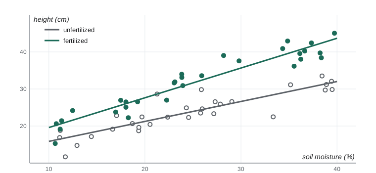
Categorical explanatory variables enter a regression through indicator (dummy) variables that equal 1 for one category and 0 otherwise. A variable with k categories needs k − 1 indicators; the omitted category is the reference, and each indicator’s coefficient is the difference from it, holding other variables constant. For example, a model for plant height with a fertilizer indicator (1 = fertilized) and soil moisture estimates the fertilizer effect at any fixed moisture level.

That model assumes the fertilizer effect is the same at every moisture level, giving parallel lines. An interaction term, the product of the two variables, allows the effect of one variable to depend on the level of another, giving lines with different slopes. Interactions are common in biology: a drug may work better in younger patients; a fertilizer may help only when water is sufficient. When an interaction is present, the main-effect coefficients describe effects at the reference or zero level of the other variable and must be interpreted with care. Centring continuous variables at their means before forming products makes main effects easier to interpret.

import numpy as np
rng = np.random.default_rng(1525)

def fit(X, y):
    X = np.column_stack([np.ones(len(y)), X])
    b, *_ = np.linalg.lstsq(X, y, rcond=None)
    return b

# Invented greenhouse trial: height (cm) vs soil moisture (%), with or without fertilizer
moist = rng.uniform(10, 40, 60)
fert = np.repeat([0, 1], 30)
height = 12 + 0.5*moist + fert*(-2 + 0.35*moist) + rng.normal(0, 2.5, 60)

m = moist - moist.mean()                       # moisture minus its mean
b = fit(np.column_stack([m, fert, m*fert]), height)
print(f"intercept (unfertilized, mean moisture) = {b[0]:.2f} cm")
print(f"moisture slope, unfertilized            = {b[1]:.3f} cm per %")
print(f"fertilizer effect at mean moisture      = {b[2]:.2f} cm")
print(f"extra moisture slope with fertilizer    = {b[3]:.3f} cm per %")
for x in (15, 25, 35):
    print(f"fertilizer effect at {x}% moisture = {b[2] + b[3]*(x - moist.mean()):.1f} cm")

intercept (unfertilized, mean moisture) = 23.89 cm
moisture slope, unfertilized            = 0.538 cm per %
fertilizer effect at mean moisture      = 7.67 cm
extra moisture slope with fertilizer    = 0.265 cm per %
fertilizer effect at 15% moisture = 5.1 cm
fertilizer effect at 25% moisture = 7.7 cm
fertilizer effect at 35% moisture = 10.3 cm

Multicollinearity

When explanatory variables are strongly correlated with each other, multicollinearity makes it hard to separate their effects. The overall fit and predictions may be fine, but individual coefficients become unstable, with large standard errors, and can change dramatically when a variable is added or removed. The variance inflation factor (VIF) for a variable is 1/(1 − R²_j), where R²_j comes from regressing that variable on all the other explanatory variables. A VIF of 1 means no inflation; values above about 5 to 10 suggest serious collinearity.

import numpy as np
rng = np.random.default_rng(1526)

def r2(X, y):
    X = np.column_stack([np.ones(len(y)), X])
    b, *_ = np.linalg.lstsq(X, y, rcond=None)
    r = y - X @ b
    return 1 - r @ r / np.sum((y - y.mean())**2)

def vif(X):
    return [1/(1 - r2(np.delete(X, j, axis=1), X[:, j])) for j in range(X.shape[1])]

# Invented fish data: length, mass and age are strongly related
age = rng.uniform(1, 8, 50)
length = 12 + 5*age + rng.normal(0, 2, 50)
mass = 0.01*length**3 * np.exp(rng.normal(0, 0.05, 50))
water_temp = rng.normal(12, 2, 50)
X = np.column_stack([age, length, mass, water_temp])
for name, v in zip(["age", "length", "mass", "water temp"], vif(X)):
    print(f"VIF {name:10s} = {v:6.1f}")

VIF age        =   20.0
VIF length     =   29.2
VIF mass       =   14.1
VIF water temp =    1.1

Remedies include dropping one of a set of redundant variables, combining them into an index, collecting data that break the correlation (in an experiment, by design), or accepting that the data cannot separate the effects and interpreting the set jointly.

Choosing a model

With many candidate variables, which should be included? The answer depends on the goal. For explanation or estimating a particular effect, variables should be chosen on scientific grounds before seeing the data: include known confounders, avoid variables that lie on the causal path between exposure and outcome, and pre-register the model if possible. For prediction, the goal is to predict new data well, and models should be compared on how they perform on data not used to fit them.

Information criteria such as the Akaike information criterion (AIC) balance fit against complexity: AIC = n ln(RSS/n) + 2k for a regression with k parameters, up to a constant, and lower values are better. Differences of less than about 2 between models are not meaningful. Cross-validation, repeatedly fitting the model to part of the data and testing it on the rest, estimates predictive accuracy directly.

Automated stepwise selection, which adds or removes variables one at a time based on p-values, is widely used but has serious problems: the selected coefficients are biased away from zero, their standard errors and p-values are too small because they ignore the selection process, and the chosen model often fails to replicate. Using AIC in place of p-values does not remove these problems. Any model chosen by searching the data should be described as exploratory and, ideally, tested on new data.

import numpy as np
rng = np.random.default_rng(1527)

def rss(X, y):
    X = np.column_stack([np.ones(len(y)), X]) if X is not None else np.ones((len(y), 1))
    b, *_ = np.linalg.lstsq(X, y, rcond=None)
    r = y - X @ b
    return r @ r, X.shape[1]

def aic(X, y):
    s, k = rss(X, y); n = len(y)
    return n*np.log(s/n) + 2*k

def cv_error(X, y, folds=5):
    idx = rng.permutation(len(y)); err = 0.0
    for f in np.array_split(idx, folds):
        train = np.setdiff1d(idx, f)
        Xt = np.column_stack([np.ones(train.size), X[train]])
        b, *_ = np.linalg.lstsq(Xt, y[train], rcond=None)
        Xv = np.column_stack([np.ones(f.size), X[f]])
        err += np.sum((y[f] - Xv @ b)**2)
    return err/len(y)

n = 60
x1, x2 = rng.normal(size=n), rng.normal(size=n)
noise = rng.normal(size=(n, 8))                  # eight irrelevant variables
y = 2 + 1.5*x1 + 0.8*x2 + rng.normal(0, 1.5, n)

models = {"x1": x1[:, None], "x1 + x2": np.column_stack([x1, x2]),
          "x1 + x2 + 8 noise": np.column_stack([x1, x2, noise])}
for name, X in models.items():
    print(f"{name:18s}: AIC = {aic(X, y):6.1f}, 5-fold CV mean squared error = {cv_error(X, y):.2f}")

x1                : AIC =   72.8, 5-fold CV mean squared error = 3.57
x1 + x2           : AIC =   57.8, 5-fold CV mean squared error = 2.51
x1 + x2 + 8 noise : AIC =   61.8, 5-fold CV mean squared error = 2.76

Regression diagnostics

Multiple regression relies on the same assumptions as simple regression, and the same residual plots check them: residuals against fitted values for curvature and non-constant variance, residuals against each explanatory variable for missed non-linearity, a normal Q–Q plot of residuals, and residuals in time or spatial order for dependence. Two further quantities identify individual observations that deserve attention.

Leverage measures how unusual an observation’s combination of explanatory variables is; points with high leverage have the potential to pull the fitted surface towards themselves. Cook’s distance combines leverage with the size of the residual to measure how much the fitted coefficients change when the observation is removed. A common rule flags Cook’s distances above 4/n for inspection. Influential points are not automatically errors, but conclusions that depend on one or two observations are fragile.

import numpy as np
rng = np.random.default_rng(1528)
n = 30
x = rng.uniform(0, 10, n)
y = 3 + 0.6*x + rng.normal(0, 1, n)
x = np.append(x, 20.0); y = np.append(y, 4.0)    # one point far out in x, off the trend

X = np.column_stack([np.ones(x.size), x])
H = X @ np.linalg.inv(X.T @ X) @ X.T
lev = np.diag(H)
b = np.linalg.lstsq(X, y, rcond=None)[0]
e = y - X @ b
k = X.shape[1]
s2 = e @ e / (x.size - k)
cooks = e**2/(k*s2) * lev/(1 - lev)**2
i = int(np.argmax(cooks))
print(f"slope with all points      = {b[1]:.3f}")
print(f"most influential point: x = {x[i]:.1f}, leverage = {lev[i]:.2f}, Cook's D = {cooks[i]:.2f} (flag above {4/x.size:.2f})")
b2 = np.linalg.lstsq(np.delete(X, i, axis=0), np.delete(y, i), rcond=None)[0]
print(f"slope without that point   = {b2[1]:.3f}")

slope with all points      = 0.321
most influential point: x = 20.0, leverage = 0.45, Cook's D = 8.97 (flag above 0.13)
slope without that point   = 0.677

Reporting a regression

A good regression report states the response and explanatory variables with units, how the variables were chosen, the sample size, each coefficient with its standard error or confidence interval, R² or adjusted R², and the checks made on the assumptions. Coefficients should be interpreted in context, with the “holding other variables constant” qualifier, and any transformations should be explained so that readers can interpret the effects on the original scale.