Correlation and simple linear regression

Much of science is about relationships between quantitative variables: how enzyme activity depends on temperature, how tree height relates to diameter, how instrument response varies with concentration. Correlation measures the strength of a linear association between two variables. Regression goes further, describing how one variable changes with another by fitting a line that can be used for prediction. This lesson covers both, with an emphasis on calibration curves, which every laboratory scientist uses, and on the checks that keep regression honest.

Scatterplots first

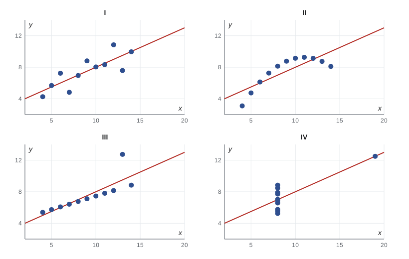
Every analysis of two quantitative variables should begin with a scatterplot, with the explanatory variable (the one that might explain or predict) on the horizontal axis and the response on the vertical axis. Look for the direction of the association (positive or negative), its form (linear or curved), its strength (how tightly the points cluster), and any unusual points. In 1973 the statistician Francis Anscombe published four small data sets with identical means, variances, correlations and regression lines, but completely different scatterplots: one linear, one curved, one with an outlier, and one in which a single point created the whole relationship. Summary statistics alone can hide everything that matters.

The correlation coefficient

The Pearson correlation coefficient r measures the strength and direction of a linear relationship. It is the average product of the standardized values of x and y:

r lies between −1 and +1. Values near ±1 indicate points close to a straight line; values near 0 indicate no linear relationship. r has no units and does not change if either variable is rescaled, so it is the same whether temperature is in degrees Celsius or Fahrenheit. It is symmetric: the correlation of x with y equals that of y with x.

Three warnings apply. First, r measures only *linear* association: a perfect U-shaped relationship can have r = 0. Second, r is sensitive to outliers, as Anscombe’s third and fourth data sets show. Third, and most important, correlation does not imply causation. Two variables may be correlated because one causes the other, because both are caused by a third (a confounder), or by coincidence. Ice cream sales and drownings are correlated because both rise in hot weather.

The test of H₀: ρ = 0, where ρ is the population correlation, uses t = r√(n − 2)/√(1 − r²) with n − 2 degrees of freedom. When data are skewed or contain outliers, the Spearman rank correlation, which is Pearson’s r applied to the ranks, measures any monotonic association and is more robust.

import numpy as np
from scipy import stats
rng = np.random.default_rng(1522)

# Invented: diameter at breast height (cm) and height (m) for 25 white spruce
dbh = np.round(rng.uniform(10, 50, 25), 1)
height = np.round(4 + 0.55*dbh - 0.004*dbh**2 + rng.normal(0, 1.5, 25), 1)

pr = stats.pearsonr(dbh, height)
sr = stats.spearmanr(dbh, height)
print(f"Pearson r = {pr.statistic:.3f}, p = {pr.pvalue:.2g}")
ci = pr.confidence_interval(0.95)
print(f"95% CI for rho: {ci.low:.3f} to {ci.high:.3f}")
print(f"Spearman rho = {sr.statistic:.3f}")

Pearson r = 0.868, p = 1.9e-08
95% CI for rho: 0.720 to 0.941
Spearman rho = 0.814

The least-squares regression line

A regression line ŷ = b₀ + b₁x describes how the mean response changes with x. The least-squares line is the one that minimizes the sum of squared vertical distances from the points to the line. These vertical distances, observed minus predicted, are the residuals. The slope and intercept have simple formulas:

The slope b₁ is the estimated change in the mean of y for a one-unit increase in x, in the units of y per unit of x. The intercept b₀ is the predicted value at x = 0, which may be meaningless if x = 0 lies outside the data. The line always passes through (x̄, ȳ). Unlike correlation, regression is not symmetric: regressing y on x gives a different line from regressing x on y, because each minimizes errors in a different direction.

The coefficient of determination, R², equals r² in simple regression. It is the proportion of the variation in y explained by the linear relationship with x. An R² of 0.81 means that 81 per cent of the variance in y is accounted for by x, and 19 per cent remains in the residuals.

Inference for the slope

The regression model assumes that, for each x, the responses are normally distributed around a mean β₀ + β₁x with constant standard deviation σ, and that observations are independent.

σ is estimated by the residual standard error s = √(Σ residuals²/(n − 2)). The standard error of the slope is s/(s_x√(n − 1)), and the t statistic b₁/SE(b₁) with n − 2 degrees of freedom tests H₀: β₁ = 0, no linear relationship. A confidence interval for the slope, b₁ ± t* SE(b₁), is usually more useful than the test, because it shows how steep the relationship might be.

Calibration curves

Instrumental analysis in chemistry, biochemistry and environmental science relies on calibration: measuring the instrument response for standards of known concentration, fitting a regression line, and then using the line in reverse to estimate the concentration of unknown samples from their responses. This inverse prediction has its own uncertainty, which depends on the scatter about the line, the number of standards, the number of replicate readings of the unknown, and how far the unknown lies from the centre of the standards.

import numpy as np
from scipy import stats

# Invented calibration: absorbance at 540 nm for nitrite standards (mg/L)
conc = np.array([0.0, 0.0, 0.2, 0.2, 0.4, 0.4, 0.6, 0.6, 0.8, 0.8, 1.0, 1.0])
absb = np.array([0.004, 0.009, 0.181, 0.173, 0.352, 0.361, 0.538, 0.527,
                 0.712, 0.704, 0.889, 0.871])
fit = stats.linregress(conc, absb)
n = conc.size
resid = absb - (fit.intercept + fit.slope*conc)
s = np.sqrt(np.sum(resid**2)/(n - 2))
tstar = stats.t.ppf(0.975, n - 2)
print(f"slope = {fit.slope:.4f} AU per mg/L (SE {fit.stderr:.4f}), intercept = {fit.intercept:.4f}")
print(f"R^2 = {fit.rvalue**2:.5f}, residual SE = {s:.4f} AU")
print(f"95% CI for slope: {fit.slope - tstar*fit.stderr:.4f} to {fit.slope + tstar*fit.stderr:.4f}")

# Inverse prediction for an unknown read in triplicate
y0 = np.array([0.455, 0.462, 0.449]); m = y0.size
x0 = (y0.mean() - fit.intercept)/fit.slope
sxx = np.sum((conc - conc.mean())**2)
se_x0 = (s/fit.slope)*np.sqrt(1/m + 1/n + (y0.mean() - absb.mean())**2/(fit.slope**2*sxx))
print(f"unknown: {x0:.3f} mg/L, 95% CI {x0 - tstar*se_x0:.3f} to {x0 + tstar*se_x0:.3f} mg/L")

slope = 0.8766 AU per mg/L (SE 0.0052), intercept = 0.0051
R^2 = 0.99964, residual SE = 0.0062 AU
95% CI for slope: 0.8650 to 0.8883
unknown: 0.514 mg/L, 95% CI 0.503 to 0.524 mg/L

A very high R², such as 0.999, is typical of a good calibration, but R² alone is not proof of linearity: a slightly curved response can still give R² above 0.99. Analysts should inspect the residuals, which should scatter randomly around zero, and should not extrapolate beyond the highest standard, where detector saturation often causes curvature. The limit of detection, the smallest concentration that can be reliably distinguished from zero, is commonly estimated as about three times the standard deviation of blank responses divided by the slope.

Confidence and prediction intervals

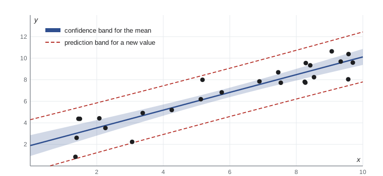
Regression supports two different kinds of interval at a given x. A confidence interval for the mean response estimates where the average y lies for all units with that x. A prediction interval estimates where a single new observation will fall. The prediction interval is always wider, because it includes the scatter of individual points around the line as well as the uncertainty in the line itself. Both are narrowest at x̄ and widen towards the ends of the data.

Residual plots and model checking

The assumptions of linearity, constant variance, normality and independence are checked mainly through the residuals. A residual plot graphs residuals against fitted values or against x. A random, even band around zero supports the model. A curved pattern means the relationship is not linear. A funnel shape, with residuals spreading out as fitted values increase, means the variance is not constant, a common pattern for concentrations and counts. A normal Q–Q plot of the residuals checks normality, which matters mainly for small samples and for prediction intervals. Independence is a matter of design, but a plot of residuals in time order can reveal drift in an instrument.

Transformations

Many biological and physical relationships are multiplicative rather than additive, and become linear after taking logarithms. Body mass and metabolic rate across species follow a power law, B = aM^b, which becomes log B = log a + b log M; the slope b of the log–log regression estimates the scaling exponent, famously close to 3/4 across many groups of organisms. Exponential growth or decay, such as bacterial counts or radioactive activity, becomes linear on a log scale of the response. Transformations can also stabilize variance and make residuals more normal.

import numpy as np
from scipy import stats
rng = np.random.default_rng(1523)

# Invented: body mass (kg) and basal metabolic rate (W) for 20 mammal species
mass = np.round(10**rng.uniform(-1.5, 3, 20), 3)
bmr = np.round(3.4*mass**0.75 * np.exp(rng.normal(0, 0.15, 20)), 2)

raw = stats.linregress(mass, bmr)
log = stats.linregress(np.log10(mass), np.log10(bmr))
print(f"raw scale:     R^2 = {raw.rvalue**2:.3f}")
print(f"log-log scale: slope = {log.slope:.3f} (SE {log.stderr:.3f}), R^2 = {log.rvalue**2:.3f}")
print(f"estimated a = {10**log.intercept:.2f} W per kg^b")

raw scale:     R^2 = 0.984
log-log scale: slope = 0.776 (SE 0.010), R^2 = 0.997
estimated a = 3.05 W per kg^b

The raw-scale R² looks impressive, but it is misleading: with masses spanning more than four orders of magnitude, the few largest species dominate the fit, and the residuals fan out as mass increases. On the log–log scale the points are evenly spread, the residuals have constant variance, and the slope of about 0.78 is close to the exponent of 0.75 used to generate the data. The standard error of 0.010 is probably optimistic for real species, because related species are not independent observations, a problem that comparative biologists address with phylogenetic methods.

Regression pitfalls

Extrapolation, predicting outside the range of x in the data, is risky because the relationship may change. Influential points, especially those with extreme x values, can pull the line towards themselves; it is good practice to fit the model with and without them and report both if the conclusions differ. Regression to the mean occurs whenever two measurements are imperfectly correlated: subjects selected for extreme first measurements will, on average, be less extreme the second time, even with no intervention. Francis Galton, who coined the term regression, observed it in the heights of parents and their adult children. It is a frequent source of spurious treatment effects in studies that enrol subjects because of extreme baseline values without a control group. Finally, a regression on observational data describes association, not the effect of changing x, unless confounders are accounted for, a task that lesson 11 begins.