
STAT-141 · Lesson 7 of 12 · 25 min
Probability
Probability is the language of uncertainty. When a weather forecast says a 30 per cent chance of rain, when a doctor says a test is 95 per cent accurate, when an insurer prices a policy, or when a pollster reports a margin of error, they are all using probability. It is also the foundation of statistical inference: to judge whether a sample result could be due to chance, we need to know how chance behaves. This lesson introduces the basic rules of probability, conditional probability and independence, Bayes' theorem with its surprising lessons about medical tests, and the counting methods behind lottery odds.
What probability means
Toss a coin a few times and the results look haphazard: heads, tails, tails, heads, heads, heads. Toss it thousands of times and the proportion of heads settles down close to one half. This is the frequency interpretation of probability: the probability of an outcome is the proportion of times it would occur in a very long series of repetitions under the same conditions. A process whose individual outcomes are uncertain but which shows a regular pattern over many repetitions is called a random phenomenon.
# The proportion of heads settles down as the number of tosses grows.
import random
random.seed(141)
heads = 0
for n in range(1, 100001):
    heads += random.random() < 0.5
    if n in (10, 100, 1000, 10000, 100000):
print(f"after {n:>6} tosses: proportion of heads = {heads / n:.4f}")after 10 tosses: proportion of heads = 0.4000 after 100 tosses: proportion of heads = 0.4800 after 1000 tosses: proportion of heads = 0.4930 after 10000 tosses: proportion of heads = 0.5002 after 100000 tosses: proportion of heads = 0.4987
The settling down of the long-run proportion is called the law of large numbers. It says nothing about short runs, which can be very streaky. A common error, the gambler's fallacy, is to believe that after several tails a head is 'due'. A fair coin has no memory: the chance of heads on the next toss is still one half, however many tails came before. The law of large numbers works not by balancing out past results but by swamping them with many future ones.
Some probabilities cannot be repeated in a long series: the chance that a particular start-up will succeed, or that it will snow on a specific day next month. Here probability expresses a degree of belief based on evidence, called subjective or personal probability. Forecasters, insurers and investors combine frequency data with judgment in this way. Either way, the same mathematical rules apply.
Sample spaces and events
The sample space S of a random phenomenon is the set of all possible outcomes. Rolling one die has sample space {1, 2, 3, 4, 5, 6}. Asking a randomly chosen customer which of four drinks they ordered has a sample space of four outcomes. An event is any set of outcomes, such as rolling an even number {2, 4, 6} or a customer ordering a hot drink. We write P(A) for the probability of event A.
When all outcomes in a finite sample space are equally likely, the probability of an event is simply the number of outcomes in the event divided by the number in the sample space. The chance of rolling an even number is 3/6 = 1/2. Many probabilities, however, are not based on equally likely outcomes: the probability that a randomly chosen resident commutes by car is the proportion of residents who do, 0.63 in our transit survey.
The basic rules
Every probability model obeys a few simple rules. Any probability is a number between 0 and 1: an event with probability 0 never occurs and one with probability 1 always occurs. The probabilities of all possible outcomes add to 1. The probability that an event does not occur, called its complement, is 1 minus the probability that it does: \(P(\text{not } A) = 1 - P(A)\). If two events are disjoint (mutually exclusive), meaning they cannot both happen, the probability that one or the other occurs is the sum of their probabilities: \(P(A \text{ or } B) = P(A) + P(B)\).
If events are not disjoint, adding their probabilities counts the overlap twice, so we subtract it once: the general addition rule is \(P(A \text{ or } B) = P(A) + P(B) - P(A \text{ and } B)\). In the transit survey, suppose 63 per cent of residents commute by car, 40 per cent are under 30, and 18 per cent are both. Then the probability that a randomly chosen resident commutes by car or is under 30 is 0.63 + 0.40 - 0.18 = 0.85.
| Rule | In symbols | Example |
|---|---|---|
| Range | 0 ≤ P(A) ≤ 1 | A probability of 1.2 is impossible |
| Total | All outcomes add to 1 | Car 0.63 + bus 0.16 + walk 0.09 + bicycle 0.07 + other 0.05 = 1 |
| Complement | P(not A) = 1 - P(A) | P(not by car) = 1 - 0.63 = 0.37 |
| Addition (disjoint) | P(A or B) = P(A) + P(B) | P(bus or walk) = 0.16 + 0.09 = 0.25 |
| General addition | P(A or B) = P(A) + P(B) - P(A and B) | P(car or under 30) = 0.63 + 0.40 - 0.18 = 0.85 |
| Multiplication (independent) | P(A and B) = P(A) P(B) | Two fair coins both heads: 0.5 x 0.5 = 0.25 |
Two-way tables and conditional probability
Real data often come as two-way tables that cross-classify individuals by two categorical variables. The clinic's records for 1,000 adults who were screened for high blood pressure show whether each person was a smoker and whether their reading was high.
| High reading | Normal reading | Total | |
|---|---|---|---|
| Smoker | 78 | 142 | 220 |
| Non-smoker | 152 | 628 | 780 |
| Total | 230 | 770 | 1,000 |
From the table, the probability that a randomly chosen adult has a high reading is 230/1,000 = 0.23. But suppose we know the person smokes. Then we restrict attention to the 220 smokers, of whom 78 have high readings, so the probability is 78/220 = 0.35. This is a conditional probability, written P(high | smoker) and read 'the probability of a high reading given that the person smokes'. In general, \(P(B \mid A) = \frac{P(A \text{ and } B)}{P(A)}\).
Conditional probabilities are not symmetric. P(high | smoker) = 78/220 = 0.35 is a different quantity from P(smoker | high) = 78/230 = 0.34; here they happen to be close, but in many situations they differ enormously, and confusing them is one of the most common and consequential errors in reasoning about probability. We will see a dramatic example below.
Rearranging the definition gives the general multiplication rule: \(P(A \text{ and } B) = P(A)\,P(B \mid A)\). If 22 per cent of adults smoke and 35 per cent of smokers have high readings, then 0.22 x 0.35 = 0.077, or about 7.7 per cent of all adults, are smokers with high readings, which matches 78 of 1,000 up to rounding.
Independence
Two events are independent if knowing that one occurs does not change the probability of the other: P(B | A) = P(B). For independent events the multiplication rule simplifies to \(P(A \text{ and } B) = P(A)\,P(B)\). Separate tosses of a coin are independent, as are the results of separate rolls of a die. In the screening data, smoking and high readings are not independent, because P(high | smoker) = 0.35 differs from P(high) = 0.23.
Independence is often assumed in risk calculations, sometimes wrongly. If two backup generators each fail with probability 0.01 and failures are independent, the chance that both fail is 0.0001. But if both generators depend on the same fuel supply or are serviced by the same technician, their failures are linked and the true chance could be much higher. Do not multiply probabilities unless independence is reasonable.
Bayes' theorem and medical tests
Aisha is helping the clinic understand a screening test for a condition that affects 2 per cent of the adults who are screened. The test's sensitivity, the probability of a positive result for someone who has the condition, is 90 per cent. Its specificity, the probability of a negative result for someone who does not, is 95 per cent. A patient tests positive. What is the probability that the patient actually has the condition? Most people, including many health professionals in published surveys, guess something close to 90 or 95 per cent. The correct answer is much lower.
A tree diagram organizes the calculation. Imagine 10,000 people screened. Two per cent, or 200, have the condition; of these, 90 per cent, or 180, test positive. Of the 9,800 without the condition, 5 per cent, or 490, test positive anyway (false positives). So 180 + 490 = 670 people test positive, and only 180 of them have the condition. The probability of having the condition given a positive test, called the positive predictive value, is 180/670, or about 27 per cent.
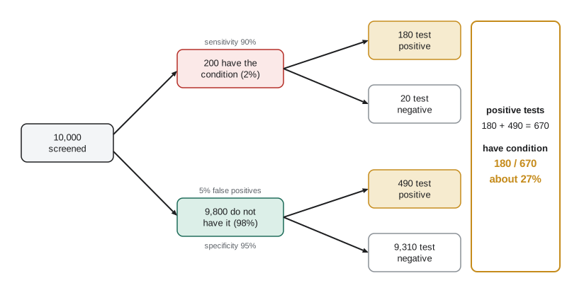
This calculation is Bayes' theorem in action. In symbols, \(P(D \mid +) = \frac{P(+ \mid D)\,P(D)}{P(+ \mid D)\,P(D) + P(+ \mid \text{not } D)\,P(\text{not } D)}\). The key insight is the role of the base rate, the prevalence of the condition. When a condition is rare, even an accurate test produces more false positives than true positives, simply because so many more people do not have the condition. That is why a positive screening result is usually followed by a more specific confirmatory test, and why screening programs for rare conditions are designed carefully.
# Bayes' theorem: positive predictive value of a screening test at different prevalences.
def ppv(prev, sens, spec):
    true_pos = sens * prev
    false_pos = (1 - spec) * (1 - prev)
    return true_pos / (true_pos + false_pos)

sens, spec = 0.90, 0.95
for prev in (0.001, 0.02, 0.10, 0.30):
    print(f"prevalence {prev:>5.1%}: P(condition | positive) = {ppv(prev, sens, spec):.1%}")
# Negative predictive value at 2% prevalence
prev = 0.02
npv = spec * (1 - prev) / (spec * (1 - prev) + (1 - sens) * prev)
print(f"at 2% prevalence, P(no condition | negative) = {npv:.2%}")prevalence 0.1%: P(condition | positive) = 1.8% prevalence 2.0%: P(condition | positive) = 26.9% prevalence 10.0%: P(condition | positive) = 66.7% prevalence 30.0%: P(condition | positive) = 88.5% at 2% prevalence, P(no condition | negative) = 99.79%
The output shows the same test with the same sensitivity and specificity giving a positive predictive value of under 2 per cent when the condition is very rare and over 85 per cent when it is common. A negative result, on the other hand, is very reassuring when the condition is rare. The same logic applies far beyond medicine: spam filters, fraud detection systems, airport screening and drug testing in the workplace all face the base-rate problem.
Counting outcomes
When outcomes are equally likely, probability calculations reduce to counting. The multiplication principle says that if one choice can be made in m ways and a second, independent choice in n ways, the two together can be made in m x n ways. A café offering 4 sizes, 6 drinks and 3 milk options has 4 x 6 x 3 = 72 possible orders.
Arranging k items in order from n distinct items gives a permutation, and there are \(n \times (n-1) \times \cdots \times (n-k+1)\) of them. Choosing k items from n when order does not matter gives a combination, and the number of combinations is \(\binom{n}{k} = \frac{n!}{k!\,(n-k)!}\), read 'n choose k', where \(n! = n \times (n-1) \times \cdots \times 1\). Choosing 3 committee members from 10 people can be done in \(\binom{10}{3} = 120\) ways.
Lottery odds come straight from combinations. In the classic draw of Lotto 6/49, sold across Canada, players choose 6 numbers from 1 to 49, and the jackpot requires matching all 6 numbers drawn. The number of possible combinations is \(\binom{49}{6} = 13{,}983{,}816\), so a single ticket's chance of matching all six is about 1 in 14 million. The game has been revised over the years, including the addition of a separate guaranteed-prize draw, but the odds for the six-number match are fixed by this count.
# Lottery odds by counting combinations: Lotto 6/49 classic draw.
from math import comb
total = comb(49, 6)
print(f"possible tickets: {total:,}")
print(f"chance of matching all 6 with one ticket: 1 in {total:,} = {1 / total:.2e}")
# Matching exactly 3 of the 6 winning numbers
ways3 = comb(6, 3) * comb(43, 3)
print(f"chance of matching exactly 3: {ways3 / total:.4f} (about 1 in {total / ways3:.0f})")
# Buying a ticket for every draw (2 per week) for 50 years
draws = 2 * 52 * 50
print(f"chance of ever winning the jackpot with one ticket per draw for 50 years: {1 - (1 - 1 / total) ** draws:.5f}")possible tickets: 13,983,816 chance of matching all 6 with one ticket: 1 in 13,983,816 = 7.15e-08 chance of matching exactly 3: 0.0177 (about 1 in 57) chance of ever winning the jackpot with one ticket per draw for 50 years: 0.00037
Numbers this small are hard to grasp. Even a person who bought a ticket for every draw for fifty years would have only a tiny chance of ever winning the jackpot. Lesson 8 adds the idea of expected value, which shows why lotteries are a reliable way for governments to raise money and an unreliable way for players to make it.
Worked problem
Reading a two-way table
Of 500 café customers surveyed, 300 use the loyalty app. Of the app users, 210 visit at least weekly; of the 200 non-users, 80 visit at least weekly. Find P(weekly), P(weekly | app user), P(app user | weekly), and decide whether app use and weekly visits are independent.
Show solution
- Weekly visitors: 210 + 80 = 290, so P(weekly) = 290/500 = 0.58.
- P(weekly | app user) = 210/300 = 0.70.
- P(app user | weekly) = 210/290 = 0.72.
- Since P(weekly | app user) = 0.70 differs from P(weekly) = 0.58, the events are not independent: app users are more likely to visit weekly.
- This association does not show that the app causes more visits; loyal customers may have been the first to join (lesson 2).
Answer: P(weekly) = 0.58, P(weekly | app) = 0.70 and P(app | weekly) = 0.72; the events are associated, not independent, but the data cannot show cause.
Common mistakes
MistakeBelieving a result is "due" after a streak (the gambler's fallacy).
InsteadIndependent trials have no memory; the probability is the same on every trial.
MistakeAdding probabilities of events that can happen together.
InsteadSubtract the overlap: P(A or B) = P(A) + P(B) - P(A and B).
MistakeConfusing P(A | B) with P(B | A).
InsteadIdentify which event is given; the two can be very different.
MistakeIgnoring the base rate when interpreting a positive test.
InsteadUse Bayes' theorem or a tree diagram with the prevalence.
MistakeMultiplying probabilities of events that are not independent.
InsteadUse the general multiplication rule P(A and B) = P(A) P(B | A).
Summary and key terms
- Probability describes the long-run proportion of times an outcome occurs; the law of large numbers says proportions settle down over many trials.
- Probabilities lie between 0 and 1, sum to 1 over all outcomes, and obey complement and addition rules.
- Conditional probability P(B | A) restricts attention to cases where A occurs; P(B | A) and P(A | B) are different.
- Independent events satisfy P(A and B) = P(A) P(B); do not assume independence without reason.
- Bayes' theorem shows that a positive result from an accurate test can still be more likely false than true when the condition is rare.
- Counting with the multiplication principle, permutations and combinations gives probabilities for equally likely outcomes, such as lottery odds.
- probability
- The long-run proportion of times an outcome would occur in many repetitions.
- law of large numbers
- The principle that the proportion of an outcome in many trials gets close to its probability.
- sample space
- The set of all possible outcomes of a random phenomenon.
- event
- A set of outcomes.
- complement
- The event that A does not occur, with probability 1 - P(A).
- disjoint events
- Events that cannot occur together.
- conditional probability
- The probability of an event given that another event has occurred.
- independent events
- Events for which knowing one occurred does not change the probability of the other.
- Bayes' theorem
- A rule for reversing conditional probabilities using base rates.
- positive predictive value
- The probability that a person with a positive test result has the condition.
- combination
- A selection of items in which order does not matter.
Practice problems
Work each problem on paper first, then reveal the answer to check.
A fair die is rolled. What is the probability of a number greater than 4?
Show answer
2/6 = 1/3.
If P(A) = 0.35, what is P(not A)?
Show answer
0.65.
P(A) = 0.5, P(B) = 0.4 and P(A and B) = 0.2. Find P(A or B). Are A and B independent?
Show answer
0.7; yes, because 0.5 x 0.4 = 0.2.
Using the screening table, find P(smoker | normal reading).
Show answer
142/770 = 0.18.
A coin lands tails five times in a row. What is the probability of heads on the next toss?
Show answer
0.5.
How many ways can 2 flavours be chosen from 8 (order not important)?
Show answer
8 choose 2 = 28.
A test has sensitivity 99 per cent and specificity 99 per cent for a condition with prevalence 1 in 1,000. Is a positive result likely to be correct?
Show answer
No: about 1 positive in 11 is true (PPV about 9 per cent).
Why might two backup systems fail together more often than independence predicts?
Show answer
They may share a common cause, such as the same power supply or maintenance error.
Lesson quiz · 5 questions
Score 60% or more to complete this lesson.
Create a free account to save your progress, take quizzes and earn a certificate.