
STAT-141 · Lesson 5 of 12 · 23 min
The normal distribution
Many quantitative variables have histograms with a similar shape: a single peak in the middle, falling off symmetrically on both sides in a smooth bell. Adult heights within one sex, scores on large standardized tests, the weights of packaged products from a well-run filling machine and errors in repeated measurements all come close to it. The mathematical model for this shape is the normal distribution. It is the most important distribution in statistics, partly because so many variables are roughly normal and, more importantly, because averages of almost any variable become normal when samples are large, a fact we meet in lesson 9.
From histograms to density curves
Imagine a histogram of thousands of observations with very narrow bins. As the bins shrink and the number of observations grows, the outline of the bars approaches a smooth curve. A density curve is such a smooth curve, scaled so that the total area under it is exactly 1. The area under the curve between two values then gives the proportion of observations that fall between them. Density curves are idealized descriptions: real data never follow one exactly, but a good curve describes the pattern well enough to be useful.
The mean of a density curve is its balance point, and the median is the point that splits the area in half. For a symmetric curve they coincide in the middle; for a right-skewed curve the mean sits to the right of the median, just as with data. We use the Greek letters \(\mu\) (mu) for the mean and \(\sigma\) (sigma) for the standard deviation of a model or population, to distinguish them from the sample statistics \(\bar{x}\) and \(s\).
The normal curve
A normal distribution is described completely by two numbers: its mean \(\mu\), which locates the centre, and its standard deviation \(\sigma\), which controls the spread. We write \(N(\mu, \sigma)\). Changing the mean slides the curve left or right without changing its shape; increasing the standard deviation makes the curve lower and wider. All normal curves have the same overall shape: symmetric, single-peaked and bell-shaped, with tails that extend forever in both directions but become very thin.
On a normal curve the standard deviation has a visual meaning. The points one standard deviation either side of the mean are where the curve changes from bending downward (around the peak) to bending upward (in the tails). Those points are called inflection points, and if you sketch a normal curve you can mark them by eye.
The 68–95–99.7 rule
For every normal distribution, about 68 per cent of observations fall within one standard deviation of the mean, about 95 per cent within two standard deviations, and about 99.7 per cent within three. This is called the empirical rule or the 68–95–99.7 rule, and it gives quick estimates without any calculation.
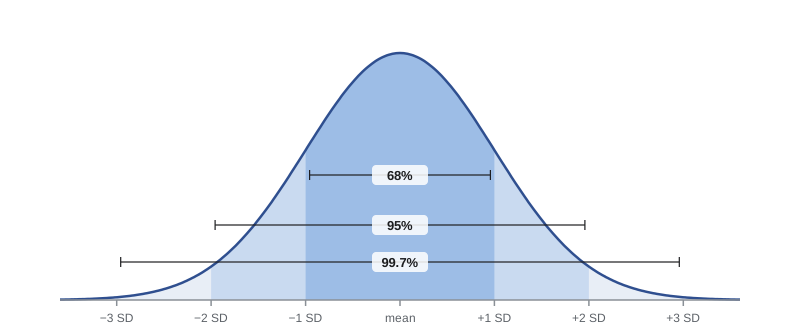
The café sells whole-bean coffee in bags labelled 340 grams. Its filling machine is set so that the weights of filled bags are approximately normal with mean 345 grams and standard deviation 3 grams. By the empirical rule, about 68 per cent of bags weigh between 342 and 348 grams, about 95 per cent between 339 and 351 grams, and nearly all between 336 and 354 grams. Since 340 grams is between 1 and 2 standard deviations below the mean, somewhat more than 2.5 per cent of bags will be under the labelled weight, which matters for consumer protection rules on packaged goods.
The standard normal distribution
Every normal distribution can be converted to one standard reference curve by computing z-scores. If \(X\) has the \(N(\mu, \sigma)\) distribution, then \(Z = \frac{X - \mu}{\sigma}\) has the standard normal distribution \(N(0, 1)\), with mean 0 and standard deviation 1. A z-score of 1.5 means one and a half standard deviations above the mean, whatever the original units were. That is why one table, or one software function, handles every normal distribution.
A standard normal table gives the area under the curve to the left of each z-value, which is the proportion of observations less than that value. Statistics software and spreadsheets compute the same areas directly; in a spreadsheet the function is usually called NORM.DIST or NORM.S.DIST. Python's built-in statistics module has a NormalDist class that does the same thing.
| z | Area to the left | Area to the right | Meaning |
|---|---|---|---|
| -2.0 | 0.0228 | 0.9772 | About 2.3 per cent of values are more than 2 SD below the mean |
| -1.0 | 0.1587 | 0.8413 | About 16 per cent are more than 1 SD below |
| 0.0 | 0.5000 | 0.5000 | Half are below the mean |
| 1.0 | 0.8413 | 0.1587 | About 84 per cent are below 1 SD above |
| 1.645 | 0.9500 | 0.0500 | The 95th percentile |
| 1.96 | 0.9750 | 0.0250 | Leaves 2.5 per cent in the upper tail |
| 2.0 | 0.9772 | 0.0228 | About 97.7 per cent are below 2 SD above |
Finding proportions
To find the proportion of a normal distribution in some range, follow four steps. State the problem in terms of the variable. Standardize the boundary values by converting them to z-scores. Find the areas from a table or software. Answer the question in context. Drawing a quick sketch of the curve with the region shaded prevents most mistakes, especially confusion between areas to the left and to the right.
# Proportions from a normal model of coffee bag weights: N(345, 3) grams.
from statistics import NormalDist
bags = NormalDist(mu=345, sigma=3)
print(f"P(weight < 340 g)         = {bags.cdf(340):.4f}")
print(f"P(weight > 350 g)         = {1 - bags.cdf(350):.4f}")
print(f"P(342 g < weight < 348 g) = {bags.cdf(348) - bags.cdf(342):.4f}")
z = (340 - 345) / 3
print(f"z-score of 340 g = {z:.2f}; standard normal area to the left = {NormalDist().cdf(z):.4f}")P(weight < 340 g) = 0.0478 P(weight > 350 g) = 0.0478 P(342 g < weight < 348 g) = 0.6827 z-score of 340 g = -1.67; standard normal area to the left = 0.0478
About 4.8 per cent of bags weigh less than 340 grams, which is more than the café wants. It has two choices: raise the mean fill, which gives away more coffee, or reduce the standard deviation by maintaining the machine better. Reducing variability is usually the smarter choice, a theme of quality improvement programs such as Six Sigma.
Working backward: percentiles
Sometimes you know the proportion and want the value. The pth percentile of a distribution is the value with p per cent of observations below it. To find a percentile of a normal distribution, find the z-value with the right area to its left, then convert back to the original units with \(x = \mu + z\sigma\).
# Working backward from a proportion to a value.
from statistics import NormalDist
bags = NormalDist(345, 3)
print(f"90th percentile of bag weight: {bags.inv_cdf(0.90):.1f} g")
# What mean fill would make only 1% of bags weigh less than 340 g, keeping sigma = 3?
z01 = NormalDist().inv_cdf(0.01)
print(f"z for the lowest 1%: {z01:.3f}; required mean = 340 - z * 3 = {340 - z01 * 3:.1f} g")
# Or keep the mean at 345 and find the sigma that achieves the same goal
print(f"required sigma with mean 345: {(340 - 345) / z01:.2f} g")90th percentile of bag weight: 348.8 g z for the lowest 1%: -2.326; required mean = 340 - z * 3 = 347.0 g required sigma with mean 345: 2.15 g
The output shows the café's choices concretely. Keeping the standard deviation at 3 grams, it would need to raise the average fill by about 2 grams per bag; alternatively, keeping the average at 345 grams, it would need to cut the standard deviation to a little over 2 grams. Engineers can then compare the cost of extra coffee with the cost of better machine maintenance.
Percentiles of normal distributions appear in many places. Growth charts used by doctors and nurses compare a child's height and weight with percentiles for children of the same age and sex. Standardized test results are often reported as percentile ranks. Insurance and pension calculations use percentiles of lifetimes and costs.
Is the normal model appropriate?
The normal distribution is a model, and many variables are not normal. Incomes, house prices, waiting times and counts of rare events are usually skewed to the right. Using a normal model for them gives wrong answers, especially in the tails, which is often exactly where the important questions are: the proportion of households with very high expenses, or the chance of a very long wait.
Check normality by looking at a histogram or a normal probability plot (also called a normal quantile plot). In a normal probability plot each observation is plotted against the value you would expect for it if the data were normal. If the data are close to normal, the points fall close to a straight line; systematic curvature shows skewness, and points that stray far from the line at the ends indicate outliers or heavy tails. You can also compare the data with the 68–95–99.7 rule.
# Checking the 68-95-99.7 rule on two invented data sets: roughly normal vs right-skewed.
import random, statistics as st
random.seed(5)
heights = [random.gauss(170, 7) for _ in range(2000)]              # adult heights, cm
waits = [random.expovariate(1 / 12) for _ in range(2000)]          # clinic waits, minutes
for name, x in (("heights", heights), ("waits", waits)):
    m, s = st.mean(x), st.stdev(x)
    within = [sum(abs(v - m) <= k * s for v in x) / len(x) for k in (1, 2, 3)]
    below = sum(v < m - 2 * s for v in x) / len(x)
print(f"{name:8s} within 1, 2, 3 SD: {within[0]:.1%} {within[1]:.1%} {within[2]:.1%} more than 2 SD below: {below:.1%}")heights within 1, 2, 3 SD: 67.6% 95.1% 99.9% more than 2 SD below: 2.5% waits within 1, 2, 3 SD: 86.6% 95.5% 98.2% more than 2 SD below: 0.0%
The heights follow the rule closely. The waiting times do not: far more than 68 per cent fall within one standard deviation, and no waits at all lie more than two standard deviations below the mean, because waits cannot be negative while the long right tail stretches out. A normal model would badly misdescribe the waits. Lesson 9 shows that even for skewed variables like this, the mean of a large sample behaves almost normally, which is why normal calculations remain so useful.
Normal approximations
Normal curves also approximate other distributions. Counts of successes in many independent trials, such as the number of customers out of 500 who redeem a coupon, follow a binomial distribution, which lesson 8 introduces; when the number of trials is large, the binomial is close to normal. Sample means and sample proportions are close to normal in large samples. These approximations are why normal calculations show up in confidence intervals and hypothesis tests throughout the rest of the course.
Worked problem
A normal calculation from start to finish
Systolic blood pressure among adults at a community health screening is approximately normal with mean 122 mmHg and standard deviation 14 mmHg. What proportion of adults have readings of 140 or higher? What reading marks the lowest 10 per cent?
Show solution
- State the problem: find P(X ≥ 140) for X distributed N(122, 14).
- Standardize: z = (140 - 122) / 14 = 1.29.
- Find the area: the area to the left of z = 1.29 is about 0.901, so the area to the right is about 0.099.
- Answer: about 10 per cent of adults have readings of 140 or higher.
- For the lowest 10 per cent, the z-value with area 0.10 to its left is -1.28, so x = 122 + (-1.28)(14) = 104.1 mmHg.
Answer: About 9.9 per cent of adults read 140 mmHg or higher, and the lowest 10 per cent read below about 104 mmHg.
Common mistakes
MistakeApplying the 68–95–99.7 rule to clearly skewed data.
InsteadCheck a histogram or normal probability plot first; the rule holds only for roughly normal data.
MistakeConfusing the area to the left with the area to the right.
InsteadSketch the curve, shade the region you want, and subtract from 1 when needed.
MistakeForgetting to standardize before using a standard normal table.
InsteadConvert values to z-scores with z = (x - mu) / sigma.
MistakeTreating the normal model as exactly true.
InsteadIt is an approximation; it can be poor in the tails even when the middle fits well.
MistakeUsing a percentile z-value with the wrong sign.
InsteadValues below the mean have negative z-scores.
Summary and key terms
- A density curve describes a distribution as a smooth curve with total area 1; areas give proportions.
- A normal distribution is symmetric and bell-shaped, determined by its mean mu and standard deviation sigma.
- About 68, 95 and 99.7 per cent of values fall within 1, 2 and 3 standard deviations of the mean.
- Standardizing with z = (x - mu)/sigma converts any normal distribution to the standard normal N(0, 1).
- Proportions come from areas under the curve; percentiles come from working backward with x = mu + z sigma.
- Check normality with histograms and normal probability plots, and do not use normal models for strongly skewed data.
- density curve
- A smooth curve with total area 1 whose areas give proportions of observations.
- normal distribution
- A symmetric, bell-shaped distribution described by its mean and standard deviation.
- empirical rule
- The 68–95–99.7 rule for the proportions of a normal distribution within 1, 2 and 3 standard deviations of the mean.
- standard normal distribution
- The normal distribution with mean 0 and standard deviation 1.
- standardizing
- Converting a value to a z-score by subtracting the mean and dividing by the standard deviation.
- percentile
- The value below which a given percentage of observations fall.
- normal probability plot
- A graph of data against the values expected under normality; a straight line suggests a normal distribution.
- inflection point
- A point where a curve changes from bending downward to bending upward.
Practice problems
Work each problem on paper first, then reveal the answer to check.
Exam scores are N(70, 8). Between what two scores do about 95 per cent of students fall?
Show answer
54 and 86.
For the same exam, what is the z-score of 82?
Show answer
(82 - 70) / 8 = 1.5.
Using the table, what proportion of a standard normal distribution lies above z = 1?
Show answer
About 0.159.
What z-value marks the 95th percentile?
Show answer
About 1.645.
Heights are N(170, 7) cm. What height is the 84th percentile?
Show answer
About one SD above the mean: 177 cm.
Why would a normal model be poor for household income?
Show answer
Income is strongly right-skewed and cannot be negative.
In a normal probability plot the points curve upward at the right end. What does this suggest?
Show answer
A longer right tail than a normal distribution (right skew).
How can a filling machine reduce underweight packages without raising the average fill?
Show answer
By reducing the standard deviation of the fill weights.
Lesson quiz · 5 questions
Score 60% or more to complete this lesson.
Create a free account to save your progress, take quizzes and earn a certificate.