
STAT-141 · Lesson 3 of 12 · 24 min
Displaying data with graphs
Before you calculate a single average, look at your data. A good graph shows the overall pattern, the unusual values and the questions you should be asking, often in a few seconds. A bad graph can hide the story or invent one. This lesson covers the standard graphs for categorical and quantitative variables, how to describe what a graph shows, and how graphs are used to mislead.
Distributions
The distribution of a variable tells you what values it takes and how often it takes each one. For a categorical variable that means the categories and the count or percentage in each. For a quantitative variable it means the range of values and where they cluster. Almost every graph in this lesson is a picture of a distribution, and almost every summary in the next lesson is a number that describes one feature of a distribution.
Graphs for categorical variables
The transit survey asked 400 residents how they usually get to work or school. A frequency table lists each category with its count, and a relative frequency table converts counts to proportions or percentages, which makes groups of different sizes comparable.
# Frequency and relative frequency table for travel mode (invented survey of 400).
from collections import Counter
modes = ["car"] * 252 + ["bus"] * 64 + ["walk"] * 36 + ["bicycle"] * 28 + ["other"] * 20
counts = Counter(modes)
n = len(modes)
print(f"{'mode':<10}{'count':>6}{'percent':>9}")
for mode, k in counts.most_common():
    print(f"{mode:<10}{k:>6}{k / n:>9.1%}")
print(f"{'total':<10}{n:>6}{1:>9.1%}")mode count percent car 252 63.0% bus 64 16.0% walk 36 9.0% bicycle 28 7.0% other 20 5.0% total 400 100.0%
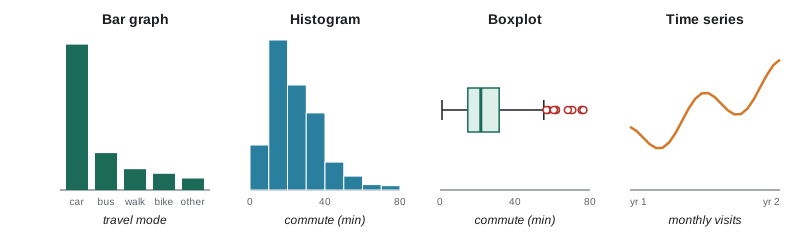
A bar graph shows each category as a bar whose height is the count or percentage. The bars are separated by gaps because the categories are distinct, and their order does not matter for nominal data, so sorting them from largest to smallest usually makes the graph easier to read. A pie chart shows each category as a slice of a circle. Pie charts work only when the categories make up a whole, and even then people judge angles and areas much less accurately than lengths, so a bar graph is almost always clearer. Pie charts are especially poor when there are many slices or when you want to compare two pies.
To compare a categorical variable across groups, use a side-by-side or segmented bar graph. For example, Lucas compared travel mode for residents under 30 and those 30 or older. A segmented bar graph shows, for each age group, a bar divided into the percentage using each mode, which makes it easy to see that younger residents are more likely to take the bus. Lesson 12 tests whether such differences could be due to chance.
Graphs for quantitative variables
A histogram groups a quantitative variable into intervals of equal width, called bins or classes, and draws a bar for each bin whose height is the count or percentage of values in it. Unlike a bar graph, the bars touch, because the bins cover a continuous range. The choice of bin width matters: too few bins hide the shape, too many make it jagged. Most software chooses a reasonable default, but it is worth trying a couple of widths.
# A text histogram of 400 invented commute times (minutes), with 10-minute bins.
import random
random.seed(141)
times = [round(random.gammavariate(3.2, 7.5)) for _ in range(400)]   # right-skewed, like real commutes
bins = range(0, 90, 10)
for lo in bins:
    k = sum(lo <= t < lo + 10 for t in times)
    print(f"{lo:>2}-{lo + 9:<3} min | {'#' * (k // 4)} {k}")
print("over 89 min:", sum(t >= 90 for t in times))0-9 min | ######### 36 10-19 min | ################################# 135 20-29 min | ########################## 104 30-39 min | ################## 74 40-49 min | ###### 26 50-59 min | #### 16 60-69 min | # 4 70-79 min | # 5 80-89 min | 0 over 89 min: 0
A stemplot, or stem-and-leaf plot, is a quick hand-made display for small data sets. Each value is split into a stem (all but the last digit) and a leaf (the last digit). The stems are written in a column and the leaves are written beside their stems, in order. A stemplot looks like a histogram turned on its side but keeps every individual value, so you can still read off the data. For example, the values 12, 15, 21, 23, 23, 28 and 34 become stems 1, 2 and 3 with leaves 2 5, 1 3 3 8 and 4.
A dotplot draws one dot for each observation above a number line, stacking dots for repeated values. Dotplots are excellent for small to moderate data sets because nothing is hidden. A boxplot, which we construct in lesson 4, summarizes a distribution with five numbers and flags unusual values; it is especially useful for comparing several groups side by side.
Describing a distribution: shape, centre, spread and outliers
When you look at a graph of a quantitative variable, describe four things. Shape: is the distribution roughly symmetric, or skewed, with a longer tail on one side? Does it have one peak (unimodal) or two (bimodal)? Centre: where is the middle of the data? Spread: how far do values range from the centre? Outliers: are there individual values that fall well outside the overall pattern?
A distribution is skewed to the right when its right tail is much longer than its left. Incomes, house prices, commute times, waiting times and the number of purchases per customer are typically right-skewed: most values are modest, but a few are very large. A distribution is skewed to the left when the left tail is longer, as with scores on an easy test or age at retirement. A symmetric distribution looks roughly the same on both sides of its centre, as many measurement errors and test scores on well-designed exams do.
| Shape | What it looks like | Everyday examples |
|---|---|---|
| Roughly symmetric | Mirror image about the centre | Adult heights within one sex, scores on a standardized test |
| Skewed right | Long tail toward large values | Household income, commute time, hospital stay length |
| Skewed left | Long tail toward small values | Scores on an easy quiz, age at death in a wealthy country |
| Bimodal | Two distinct peaks | Café visits by hour (morning and afternoon rush), heights of adults of both sexes combined |
| Uniform | Roughly flat | Last digit of phone numbers, rolls of a fair die |
Bimodal shapes often signal that two different groups have been combined. If the café's hourly sales show peaks at 8 a.m. and 3 p.m., the data mix morning commuters with afternoon students, and it might be more useful to study the two groups separately.
An outlier is a value that falls far from the rest. Outliers deserve attention, not automatic deletion. Some are errors: a commute recorded as 400 minutes may be a typing mistake for 40. Others are genuine and interesting: a customer who visited 90 times in a month may be an employee using the app, or a very loyal regular. Investigate first; then decide, and report what you decided.
Graphs over time
Data recorded at regular intervals, such as monthly sales, daily temperatures or the yearly unemployment rate, form a time series. A time series plot puts time on the horizontal axis and the variable on the vertical axis, connecting the points with lines. Look for a long-term trend (an overall rise or fall), seasonal variation (a pattern that repeats each year, week or day) and unusual movements. The café's monthly visits rise over two years, with a low point each June, when many students leave the city, and a peak each December: a trend plus seasonality.
# Monthly cafe visits (thousands) with trend and a seasonal pattern, and a 12-month moving average.
import math
visits = []
for m in range(24):
    trend = 40 + 0.6 * m
    season = 4 * math.cos(2 * math.pi * (m - 11) / 12)   # peak in December (month 11, 23)
    visits.append(round(trend + season, 1))
months = ["Jan", "Feb", "Mar", "Apr", "May", "Jun", "Jul", "Aug", "Sep", "Oct", "Nov", "Dec"]
for m in (0, 5, 11, 12, 17, 23):
    print(f"{months[m % 12]} year {m // 12 + 1}: {visits[m]:5.1f} thousand")
ma = sum(visits[12:24]) / 12
print(f"12-month average, year 2: {ma:.1f} thousand (year 1: {sum(visits[:12]) / 12:.1f})")Jan year 1: 43.5 thousand Jun year 1: 39.0 thousand Dec year 1: 50.6 thousand Jan year 2: 50.7 thousand Jun year 2: 46.2 thousand Dec year 2: 57.8 thousand 12-month average, year 2: 50.5 thousand (year 1: 43.3)
Seasonal patterns are why official statistics are often reported seasonally adjusted. Retail sales always jump in December and employment in construction always rises in summer, so agencies remove the usual seasonal swing to show whether the underlying trend is changing. When a news report says the unemployment rate rose, it usually means the seasonally adjusted rate.
Graphs that mislead
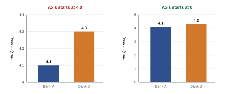
Graphs persuade because people trust what they see, and that makes them easy to abuse. The most common trick is a truncated vertical axis. If a bar graph of two interest rates, 4.1 and 4.3 per cent, starts its axis at 4.0, the second bar looks three times as tall as the first, although the rates differ by only 5 per cent of their value. For bar graphs, whose message is carried by bar length, the axis should start at zero. For line graphs that show change over time, starting away from zero can be reasonable, but the scale should be clearly labelled.
Other tricks include picture graphs in which an icon is scaled in both height and width, so that doubling a value quadruples the area; three-dimensional effects that distort the size of slices and bars; cherry-picked time windows that start at an unusual low or high; dual vertical axes with different scales that make two unrelated series appear to move together; and graphs with no labels or sources at all. When you see a graph, check the axes, the scale, the time window and the source before you accept its message.
| Trick | Effect | What to check |
|---|---|---|
| Truncated vertical axis on a bar graph | Small differences look huge | Does the axis start at zero? |
| Scaled pictograms | Area grows with the square of the value | Is only one dimension scaled? |
| 3-D pie or bar effects | Front slices look bigger | Are values labelled directly? |
| Cherry-picked time window | A trend appears or disappears | What happens with a longer window? |
| Two vertical axes | Unrelated series seem linked | Are both scales shown and sensible? |
| Cumulative totals | Always rising, hiding a slowdown | Would per-period values tell a different story? |
Choosing a graph
Match the graph to the variable and the question. One categorical variable: a bar graph (or a pie chart if the parts form a whole and there are few of them). One quantitative variable: a histogram, dotplot, stemplot or boxplot. A quantitative variable across groups: side-by-side boxplots or histograms on the same scale. Two categorical variables: a side-by-side or segmented bar graph. Two quantitative variables: a scatterplot, covered in lesson 6. A variable over time: a time series plot. Label axes with the variable name and units, give the graph a clear title, state the source and the sample size, and keep decoration to a minimum.
Colour deserves thought. Roughly one in twelve men and one in two hundred women have some form of colour vision deficiency, most often difficulty telling red from green. Using colour palettes that remain distinguishable, adding direct labels and using patterns or shapes as well as colour makes graphs readable for everyone.
Worked problem
Reading a histogram
Aisha makes a histogram of the waiting times (minutes) of 250 patients at the clinic. Most patients wait between 5 and 25 minutes, the tallest bar is at 10 to 15 minutes, a few patients wait 40 to 60 minutes, and one record shows 185 minutes. Describe the distribution.
Show solution
- Shape: unimodal and skewed to the right, with a long tail toward long waits.
- Centre: typical waits are around 10 to 15 minutes.
- Spread: most waits fall between 5 and 25 minutes, with a tail up to about 60 minutes.
- Outlier: the 185-minute record is far beyond the rest and should be checked; it might be an error (for example, a patient who left and returned) or a genuine extreme case.
Answer: A unimodal, right-skewed distribution centred near 10 to 15 minutes, mostly between 5 and 25, with one suspicious outlier at 185 minutes that needs investigation.
Common mistakes
MistakeUsing a pie chart for categories that do not make up a whole or for many small slices.
InsteadUse a bar graph, sorted from largest to smallest.
MistakeLeaving gaps between histogram bars or treating bins as categories.
InsteadHistogram bars touch because the bins cover a continuous range.
MistakeStarting a bar graph's vertical axis above zero.
InsteadStart bar graphs at zero so bar length reflects the value.
MistakeDeleting outliers without investigating them.
InsteadCheck whether each outlier is an error or a genuine value, and report your decision.
MistakeDescribing a distribution only by its centre.
InsteadDescribe shape, centre, spread and outliers.
Summary and key terms
- A distribution shows what values a variable takes and how often.
- Use bar graphs (and occasionally pie charts) for categorical variables; histograms, stemplots, dotplots and boxplots for quantitative ones.
- Describe a quantitative distribution by its shape, centre, spread and outliers.
- Right-skewed distributions, with a long upper tail, are common for money, time and counts.
- Time series plots reveal trend and seasonality; seasonal adjustment removes the usual yearly pattern.
- Check axes, scales, time windows and sources to avoid being misled by graphs.
- distribution
- The values a variable takes and how often it takes them.
- frequency table
- A table listing categories or intervals with their counts.
- bar graph
- A graph of a categorical variable with a separate bar for each category.
- histogram
- A graph of a quantitative variable using touching bars over equal-width intervals.
- stemplot
- A display that splits each value into a stem and a leaf, keeping the individual values.
- skewed to the right
- Having a longer tail toward large values.
- bimodal
- Having two distinct peaks.
- outlier
- An individual value that falls outside the overall pattern of the data.
- time series
- Measurements of a variable taken at regular intervals over time.
- seasonal adjustment
- Removing the regular seasonal pattern from a time series to reveal its trend.
Practice problems
Work each problem on paper first, then reveal the answer to check.
Which graph would you use for the number of students in each faculty?
Show answer
A bar graph, because faculty is categorical.
Why do the bars of a histogram touch?
Show answer
Because the intervals cover a continuous range of a quantitative variable.
Hospital stays have most patients staying 1 to 3 days and a few staying over a month. What shape is the distribution?
Show answer
Skewed to the right.
Write a stemplot for 31, 35, 42, 44, 44, 47, 53.
Show answer
Stems 3, 4, 5 with leaves 1 5 | 2 4 4 7 | 3.
A bar graph of two prices, 9.80 and 10.20, starts its axis at 9.50. What is wrong?
Show answer
The truncated axis makes a 4 per cent difference look much larger.
Hourly visits to an emergency department show peaks at noon and 7 p.m. What might this suggest?
Show answer
A bimodal pattern, possibly reflecting different groups or activities at different times of day.
What two features of a time series should you look for?
Show answer
A long-term trend and seasonal variation (plus any unusual movements).
Give one way to make a graph readable for people with colour vision deficiency.
Show answer
Use a colour-blind-friendly palette and add direct labels or patterns.
Lesson quiz · 5 questions
Score 60% or more to complete this lesson.
Create a free account to save your progress, take quizzes and earn a certificate.