Fans, fan laws and system curves

Every air system has one or more fans, and every balancing job ends with the fan. Branch dampers decide how the air is shared; the fan decides how much there is to share. Before Kai could set the Ashgrove library dampers, he had to understand what RTU-2's supply fan could do, what the duct system was asking of it, and what would happen when someone changed its speed. This lesson covers fan types, fan curves, system curves, the operating point where they meet, the fan laws that predict the effect of a speed change, and system effect, the hidden loss that makes many fans fall short of their rating.

Fan types

Centrifugal fans draw air into the centre of a spinning wheel and throw it outward into a scroll housing. The blades can be forward-curved, common in small packaged units and furnaces because they move a lot of air at low speed in a small housing; backward-inclined or airfoil, used in larger air handlers because they are more efficient and their power draw levels off at high flow; or radial, used for dirty or material-handling exhaust. Plenum or plug fans are centrifugal wheels without a scroll, set in a casing and discharging in all directions, common in modern air handlers. Axial fans move air straight through along the shaft and include propeller fans for exhaust and vane-axial fans for high-volume ducted systems.

Fans are belt-driven or direct-driven. A belt drive uses a motor sheave and a fan sheave, and the fan speed is set by their ratio. Changing a sheave, or adjusting an adjustable-pitch motor sheave, changes the fan speed. A direct-drive fan turns at the motor's speed and is adjusted with a variable-frequency drive or, on small fans, a multi-speed or electronically commutated motor. RTU-2 at Ashgrove has a belt-driven forward-curved supply fan with an adjustable motor sheave, which matters in lesson 9.

Fan curves

A fan's performance is shown on a fan curve, a graph from the manufacturer's tests, plotting the static or total pressure the fan develops against the airflow it delivers at a given speed and air density. For a forward-curved fan the curve is fairly flat in its working range, with a dip near the left; for a backward-inclined fan it falls more steeply. The curve usually also shows brake horsepower or shaft power, efficiency, and lines for other speeds. Fan performance can also be given as a table of airflow and pressure at each speed, the usual form in equipment submittals.

A fan curve is only valid for the conditions it was tested at: the speed, the air density and an ideal inlet and outlet arrangement defined by the test standard. In a real installation the inlet may be crowded and the outlet may have an elbow right at the fan, and the fan will not perform as rated. That loss is system effect, discussed below.

System curves and the operating point

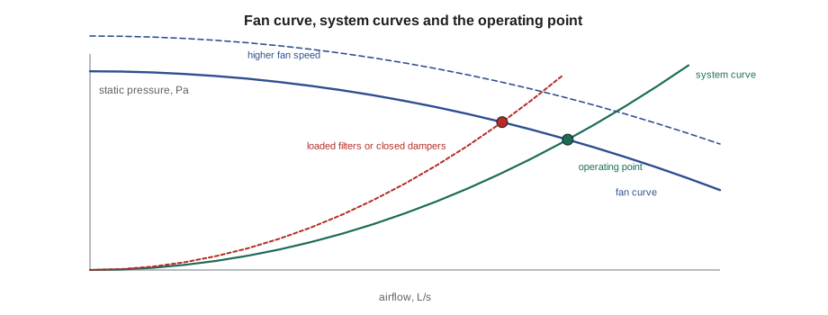
A duct system has a characteristic of its own. The pressure needed to push air through ducts, fittings, coils and filters rises roughly with the square of the airflow: double the flow and the friction and fitting losses are about four times as large. Plotted on the same graph as the fan curve, this gives a system curve, a parabola starting at zero flow and zero pressure.

The fan and the system settle at the one point that satisfies both: the airflow at which the pressure the fan develops equals the pressure the system needs. That operating point is where the curves cross. If the system has more resistance than the designer calculated, because of dirty filters, a closed damper, extra fittings or a crushed flexible duct, its curve is steeper and crosses the fan curve at a lower airflow. If it has less, the airflow is higher. Every balancing adjustment moves one curve or the other: closing a branch damper raises the system curve; speeding up the fan raises the fan curve.

# Find where a fan curve and a system curve cross (illustrative RTU-2 data at one speed)
fan = [(1000, 820), (1300, 790), (1600, 730), (1900, 640), (2200, 510)]                  # (airflow L/s, static pressure Pa)
k = 0.0003                      # system constant: dp = k * Q^2
def fan_p(q):
    for (q1, p1), (q2, p2) in zip(fan, fan[1:]):
        if q1 <= q <= q2:
            return p1 + (p2 - p1) * (q - q1) / (q2 - q1)
lo, hi = fan[0][0], fan[-1][0]
for _ in range(60):          # bisection on fan pressure minus system pressure
    mid = (lo + hi) / 2
    if fan_p(mid) - k * mid**2 > 0: lo = mid
    else: hi = mid
print(f"operating point: {mid:.0f} L/s at {k*mid**2:.0f} Pa")
k_dirty = k * 1.18           # filters loaded, about 18 percent more resistance
lo, hi = fan[0][0], fan[-1][0]
for _ in range(60):
    mid2 = (lo + hi) / 2
    if fan_p(mid2) - k_dirty * mid2**2 > 0: lo = mid2
    else: hi = mid2
print(f"with loaded filters: {mid2:.0f} L/s ({100*mid2/mid:.0f}% of clean)")

operating point: 1567 L/s at 737 Pa
with loaded filters: 1463 L/s (93% of clean)

The example shows why clean filters matter before balancing. The same fan at the same speed delivers several percent less air when the filters are loaded, enough to push a system that was marginal out of tolerance. TAB is done with clean filters, and the report records the filter pressure drop at the time of the test so the owner knows the starting condition.

The fan laws

When a fan's speed changes but nothing else does, the fan laws predict how its airflow, pressure and power change. They follow from the fact that a fan running faster moves proportionally more air through the same system, the pressure needed rises with the square of the airflow, and the power is airflow times pressure.

Here N is fan speed in revolutions per minute, Q airflow, p pressure and W power. The cube law for power is the important one for a balancer. A 10 percent increase in speed gives 10 percent more air but needs about 33 percent more power, and the motor that was comfortable at the old speed may be overloaded at the new one. Every speed increase is checked against the motor's nameplate current and power before it is made. Equally, a 20 percent reduction in speed cuts power to about half, which is why variable-speed drives save so much energy on systems that do not need full flow all the time.

The fan laws hold only when the system does not change. If dampers are moved at the same time, or if the fan is on a different part of its curve where it stalls or surges, they do not apply. They also assume the same air density; a fan moving cold winter air develops more pressure and draws more power than it does on a summer test.

# Fan laws: predict the effect of a speed change, then check the motor
n1, n2 = 1050, 1150          # fan speed before and after, rpm
q1, p1, w1 = 1520, 690, 1.55  # airflow L/s, static pressure Pa, shaft power kW
r = n2 / n1
print(f"speed ratio {r:.3f}")
print(f"airflow  {q1} -> {q1*r:.0f} L/s")
print(f"pressure {p1} -> {p1*r**2:.0f} Pa")
print(f"power    {w1} -> {w1*r**3:.2f} kW")
motor_rating = 2.24          # motor nameplate, kW
print("motor OK" if w1*r**3 <= motor_rating else "motor too small: check before changing speed")

speed ratio 1.095
airflow  1520 -> 1665 L/s
pressure 690 -> 828 Pa
power    1.55 -> 2.04 kW
motor OK

System effect

Fan ratings come from tests with smooth, straight inlet and outlet ducts. In the field, fans are crammed into units and rooms, with elbows at the outlet, plenums at the inlet and transitions right at the fan. These arrangements disturb the flow entering or leaving the wheel and reduce the fan's effective performance. The reduction is called system effect, and it shows up as a fan that seems to deliver less than its curve says at the measured pressure. The AMCA fan application manual gives factors for common arrangements, and the SMACNA and TAB references discuss them.

A typical example is an elbow bolted directly to a fan outlet. Air leaves a centrifugal fan's scroll with an uneven velocity profile, and it needs several duct diameters to even out. An elbow turning the air before that happens adds a large pressure loss that the designer did not count. Inlet problems are often worse: a fan inlet close to a wall, a casing or a sharp turn spins the air before it reaches the wheel, and the fan can lose a large share of its rated capacity. A TAB technician who finds a fan well short of its rating, with the system otherwise clean and open, looks for system effect before suggesting a larger motor.

At Ashgrove, RTU-2 sits on a roof curb with the supply dropping straight down through the roof before the first elbow, as Sean's crew installed it in SMW-310. That straight drop of about 1.5 m is good practice for system effect. The return connection, by contrast, enters the side of the unit close to a structural beam, and Marisol noted it on her design review as a possible inlet effect to check if the fan came up short.

Fans in series and parallel, and unstable operation

Large systems sometimes have more than one fan: a supply and a return fan in series around the same air, or two supply fans in parallel. Fans in parallel add their airflows at the same pressure; fans in series add their pressures at the same airflow. Supply and return fans must be balanced together, because the return fan sets the pressure in the mixing box and the building. In a VAV system, a return fan that tracks the supply fan badly can make the building strongly negative or positive, which lesson 10 discusses.

Some fans, especially forward-curved and airfoil centrifugal fans, have a region to the left of their peak pressure where operation is unstable. A fan pushed there by too much system resistance can surge, hunting back and forth with a pulsing noise, and the readings never settle. A TAB technician who sees a fan's static pressure swinging and its airflow fluctuating checks whether it is operating in that region, and the fix is to reduce the system resistance or change the speed, not to keep closing dampers.

Fan curves from the manufacturer

The curve in a submittal is a laboratory curve, measured with ideal inlet and outlet ducts on a test rig. It shows what the fan can do, not what it will do in the building. The TAB technician uses it as the starting point: find the design point on the curve, note the speed and power the manufacturer predicts there, and compare those with what is measured once the system runs. A large gap between the predicted and measured operating points is a sign of system effect, an incorrect fan, a slipping belt or a system with far more resistance than the design assumed, and each of those has a different fix.

Marisol keeps the submittal curve for RTU-2 in the job binder with the measured point marked on it in pencil, so anyone who opens the file later can see where the fan actually runs.