
ROB-460 · Lesson 3 of 12 · 32 min
Perception and localization outdoors
ROB-310 and ROB-340 developed the probabilistic tools for estimating a robot's position and building maps: Bayes filters, Kalman and particle filters, and SLAM in its many forms. Those methods assume sensors that behave roughly as modelled. Outdoors, sensors meet sunlight, rain, snow, dust, fog, vegetation, featureless fields and satellite signals that are blocked, reflected or deliberately jammed. This lesson is about the sensors and the failure modes that matter in the field, how to quantify drift when the best sensors drop out, and how robust field systems detect degradation and fall back gracefully. It refers to ROB-340 for the estimation algorithms themselves, and to CON-250 lesson 4 for the surveying side of GNSS and real-time kinematic positioning.
Satellite positioning in the field
Global navigation satellite systems (GPS, GLONASS, Galileo and BeiDou) are the backbone of outdoor localization. A single-frequency standalone receiver gives positions good to a few metres. Dual-frequency receivers remove most ionospheric delay. Real-time kinematic (RTK) positioning uses carrier-phase measurements and corrections from a nearby base station or a network to reach centimetre accuracy, which is why it is standard on autonomous tractors, haul trucks and survey robots. Precise point positioning (PPP) uses precise satellite orbit and clock products instead of a local base, converging to decimetre or better accuracy over minutes; several services now deliver PPP corrections by satellite or internet, including combined PPP-RTK products.
In Canada, Natural Resources Canada provides the free CSRS-PPP online service for post-processing and maintains the Canadian Spatial Reference System; provincial and commercial RTK networks cover most farming regions. Coverage is thinner in the North, where low satellite elevations and ionospheric disturbances near the auroral zone make high-accuracy GNSS harder.
In the field, accuracy depends as much on the environment as on the receiver. Tree canopy, steep valley walls, open-pit mine walls and buildings block satellites and reflect signals, causing multipath errors that can reach metres and loss of RTK fix. The geometry of the visible satellites is summarized by the dilution of precision (DOP); when satellites are clustered in one part of the sky, the horizontal DOP rises and so do position errors. A rule of thumb is that horizontal error is roughly HDOP times the range error per satellite.
| Positioning mode | Typical horizontal accuracy | Needs | Field limitations |
|---|---|---|---|
| Standalone single-frequency | 2 to 5 m | Receiver only | Ionospheric and multipath errors |
| Satellite-based augmentation (WAAS in North America) | about 1 m | Receiver able to use augmentation | Less useful at high latitudes |
| PPP | a few cm to 10 cm after convergence | Correction service | Convergence time of minutes; re-convergence after outages |
| RTK | 1 to 3 cm | Base station or network within tens of km and a data link | Loses fix under canopy and near walls; link dropouts |
Worked problem
Position error from poor satellite geometry
An orchard robot's receiver estimates a range error of 0.5 m per satellite with standalone dual-frequency positioning. In the open the HDOP is 0.9; between tall rows it rises to 3.5. Estimate the horizontal error in each place.
Show solution
- Open field: \( 0.9 \times 0.5 = 0.45 \) m.
- Between rows: \( 3.5 \times 0.5 = 1.75 \) m.
- Multipath from foliage may add more, so the in-row figure is optimistic.
Answer: About 0.5 m in the open but nearly 2 m between rows, which is too large for driving between rows 3 m apart without another source of positioning.
GNSS signals are extremely weak at the Earth's surface, so they are easy to jam and, with more effort, to spoof. Interference from illegal jammers, military activity and unintentional sources has been reported widely in recent years, including in regions near conflict zones where aviation and shipping have experienced large-scale disruption. Field robots that depend on GNSS should monitor signal-to-noise ratio, sudden position jumps and disagreement with inertial and odometry estimates, and treat GNSS as one input to a filter rather than as ground truth.
Dead reckoning and drift
When GNSS is unavailable, a robot falls back on dead reckoning: integrating wheel odometry, inertial measurements or visual odometry from a known start. Every dead-reckoning method drifts, and the shape of the drift matters. Random noise in a velocity measurement produces position error that grows roughly with the square root of time, like a random walk. A constant bias in a gyroscope produces a heading error that grows linearly with time, and because position is the integral of velocity in the wrong direction, the cross-track position error grows with the square of time or distance. A heading error of \( \delta\psi \) radians over a straight distance \( d \) produces a cross-track error of about \( d\,\delta\psi \).
Worked problem
Heading error and cross-track drift
A robot drives 1 km in a straight line with a heading error of 1 degree. What cross-track error results? What if the heading error grows linearly from 0 to 1 degree over the same distance because of gyro bias?
Show solution
- 1 degree = 0.01745 rad.
- Constant error: \( e = 1000 \times 0.01745 \approx 17.5 \) m.
- Linearly growing error averages half the final value along the path: \( e \approx 17.5 / 2 \approx 8.7 \) m.
Answer: About 17.5 m for a constant 1 degree error and about 8.7 m for a heading error growing to 1 degree; small angles produce large errors over long distances.
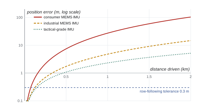
# Monte Carlo drift of wheel-odometry + gyro dead reckoning on a 2 km straight drive
import numpy as np
rng = np.random.default_rng(460)
v, dt, T = 1.0, 0.1, 2000.0                 # 1 m/s for 2000 s
steps = int(T / dt)
def run(gyro_bias_deg_h, gyro_noise_deg_rt_h, odo_scale_err, trials=300):
    b = np.radians(gyro_bias_deg_h) / 3600 * rng.choice([-1, 1], trials)
    arw = np.radians(gyro_noise_deg_rt_h) / 60      # angle random walk per sqrt(s)
    psi = np.zeros(trials); x = np.zeros(trials); y = np.zeros(trials)
    scale = 1 + odo_scale_err * rng.standard_normal(trials)
    for _ in range(steps):
        psi += b * dt + arw * np.sqrt(dt) * rng.standard_normal(trials)
        x += v * scale * np.cos(psi) * dt
        y += v * scale * np.sin(psi) * dt
    err = np.hypot(x - v * T, y)
    return np.percentile(err, 50), np.percentile(err, 95)
for name, args in {"consumer MEMS IMU": (10.0, 0.3, 0.01),
                   "industrial MEMS IMU": (1.0, 0.1, 0.005),
                   "tactical-grade IMU": (0.1, 0.02, 0.002)}.items():
    p50, p95 = run(*args)
print(f"{name:20s} median error {p50:6.1f} m 95th percentile {p95:6.1f} m ({p95/20:.2f} % of distance)")consumer MEMS IMU median error 98.5 m 95th percentile 107.8 m (5.39 % of distance) industrial MEMS IMU median error 12.1 m 95th percentile 21.2 m (1.06 % of distance) tactical-grade IMU median error 2.6 m 95th percentile 7.5 m (0.38 % of distance)
The simulation shows why IMU grade matters so much for long GNSS outages. With a consumer-grade gyro, errors after 2 km approach 100 m, about 5 per cent of the distance; an industrial unit keeps them near 10 to 20 m and a tactical-grade unit to a few metres, at a much higher price. Odometry scale error adds along-track error that grows linearly with distance. Field robots therefore combine dead reckoning with absolute corrections whenever they are available: GNSS when it returns, recognized landmarks, matching against a prior map, or terrain-relative navigation that compares sensed terrain shape with a stored elevation model.
Lidar, cameras and radar in bad weather
Lidar is the workhorse of mapping and obstacle detection, but its laser pulses are scattered and absorbed by rain, snow, fog and dust. Two effects matter. Attenuation reduces the returned power, shortening the useful range; in a uniform medium with extinction coefficient \( \alpha \) the received power falls as \( e^{-2\alpha R} \) in addition to the usual range loss. Backscatter from droplets, snowflakes and dust creates false returns close to the sensor, which can look like obstacles. Many lidars report multiple returns per pulse, and filtering by intensity, return number and the spatial pattern of points removes much of the clutter; learned filters trained on adverse-weather data sets do better still. Sensor windows also get dirty, wet or iced, so field robots often have wipers, washers, air knives or heaters, and monitor the fraction of expected returns to detect blockage.
Worked problem
Lidar range in fog
A lidar detects a 10 per cent reflective target at 100 m in clear air at the edge of its sensitivity. In moderate fog the extinction coefficient at its wavelength is about 0.02 per metre. Ignoring the change in geometric loss, what fraction of the clear-air signal returns from 100 m, and what range gives the same received power if range loss scales as \( 1/R^2 \)?
Show solution
- Two-way fog loss at 100 m: \( e^{-2 \times 0.02 \times 100} = e^{-4} \approx 0.018 \).
- At range \( R \) the received power relative to clear air at 100 m is \( (100/R)^2 e^{-0.04R} \).
- Setting this equal to 1 and solving numerically gives \( R \approx 43 \) m.
Answer: Only about 2 per cent of the signal returns from 100 m; the maximum range for that target falls to roughly 43 m, less than half the clear-air value.
Cameras suffer from glare, low light, shadows, rain on the lens and the changing appearance of vegetation through the seasons; a place-recognition model trained in summer may fail in winter. High-dynamic-range sensors, polarizing filters and active illumination help, and thermal infrared cameras see people and animals in darkness and through light smoke. Radar, especially millimetre-wave radar around 77 GHz, penetrates dust, fog, rain and snow far better than lidar or cameras, at the cost of lower angular resolution and noisy returns. Imaging radars and radar odometry have become practical for mining and off-road vehicles, where dust can make lidar nearly useless.
| Sensor | Strengths outdoors | Weaknesses outdoors | Typical mitigations |
|---|---|---|---|
| GNSS (RTK) | Absolute centimetre positions in the open | Canopy, walls, multipath, jamming | Fuse with IMU and odometry; monitor fix quality |
| Lidar | Precise 3D geometry day or night | Rain, snow, fog, dust; dirty windows | Multi-return filtering, cleaning systems, blockage monitoring |
| Cameras | Rich appearance, low cost | Lighting, glare, season changes, water on lens | HDR sensors, learned features, lens hoods and wipers |
| Thermal cameras | People and animals at night, through smoke | Low resolution, thermal crossover at dawn and dusk | Fuse with visible cameras |
| Radar | Works through dust, fog and precipitation | Low angular resolution, clutter | Imaging radar, fusion with lidar |
| IMU and wheel odometry | Always available, high rate | Drift; wheel slip on soft ground | Slip detection, absolute corrections |
Degradation-aware localization
Robust field systems do not simply fuse every sensor all the time. They estimate the health of each sensor and adapt. A mine vehicle may switch from lidar-based localization to radar and inertial navigation when dust levels rise; an orchard robot may rely on row-following with cameras when GNSS fix is lost between trees and return to RTK at the headland. Techniques include monitoring the innovation, the difference between predicted and actual measurements in a Kalman filter, and rejecting measurements whose normalized innovation squared exceeds a chi-square threshold; checking for degeneracy in lidar scan matching, which happens in long featureless tunnels and open fields where geometry does not constrain motion in every direction; and maintaining multiple hypotheses when the robot may be in one of several similar places.
Teams in the DARPA Subterranean Challenge showed the value of such resilience. Leading systems fused lidar, cameras, thermal cameras and IMUs, detected when one modality was degraded and switched estimators, and shared maps among robots when communication allowed. Many published field systems now report results across seasons, weather and lighting conditions, because a method that works on a sunny day is not yet a field method.
# Innovation gating: reject GNSS fixes that disagree with the filter prediction
import numpy as np
rng = np.random.default_rng(7)
pred = np.array([100.0, 50.0])              # predicted position (m)
P = np.diag([0.30**2, 0.30**2])             # prediction covariance
R = np.diag([0.05**2, 0.05**2])             # RTK fix covariance
S = P + R                                   # innovation covariance
gate = 9.21                                 # chi-square 99 % for 2 degrees of freedom
fixes = [pred + rng.normal(0, 0.3, 2) for _ in range(4)] + [pred + np.array([4.0, -3.0])]
for i, z in enumerate(fixes):
    nu = z - pred
    nis = float(nu @ np.linalg.solve(S, nu))
print(f"fix {i}: innovation {np.round(nu, 2)} NIS {nis:7.2f} {'accept' if nis < gate else 'reject (multipath or spoofing?)'}")fix 0: innovation [0. 0.09] NIS 0.09 accept fix 1: innovation [-0.08 -0.27] NIS 0.84 accept fix 2: innovation [-0.14 -0.3 ] NIS 1.16 accept fix 3: innovation [0.02 0.4 ] NIS 1.75 accept fix 4: innovation [ 4. -3.] NIS 270.27 reject (multipath or spoofing?)
The last fix, five metres away from the prediction, is rejected. A real system would not reject GNSS forever: if several consecutive fixes disagree consistently, the filter may be the one that is wrong, for example because the wheels were slipping, so the system needs logic to re-initialize. Designing these rules, and testing them with recorded data from real outages, is a large part of making outdoor localization dependable.
Common mistakes
MistakeTreating an RTK position as ground truth at all times.
InsteadMonitor fix type, DOP and innovations, and fuse GNSS with inertial and odometry estimates so that outages and multipath are detected.
MistakeQuoting dead-reckoning accuracy as a percentage of distance from a short test.
InsteadBias-driven drift grows faster than linearly; test over the longest expected outage and quote error at that distance.
MistakeAssuming lidar will see through dust or fog because it works at night.
InsteadLidar is degraded by particles; use radar or reduce speed, and filter backscatter returns.
MistakeFusing all sensors with fixed weights.
InsteadEstimate sensor health and adapt weights or switch estimators when a modality degrades.
MistakeTraining perception models on one season.
InsteadCollect and validate across seasons, weather and lighting conditions before deployment.
Summary and key terms
- GNSS accuracy ranges from metres standalone to centimetres with RTK, but canopy, walls and multipath degrade it in the field.
- Dilution of precision scales range errors into position errors when satellites are poorly spread.
- GNSS is vulnerable to jamming and spoofing and should be one input to a filter.
- Dead reckoning drifts; gyro bias makes cross-track error grow roughly with the square of time.
- Lidar range falls in fog, rain and dust and backscatter creates false returns; radar penetrates particles better.
- Cameras and thermal cameras face lighting and seasonal changes but add appearance and night vision.
- Degradation-aware localization monitors innovations and sensor health and switches strategies when needed.
- RTK
- Real-time kinematic GNSS positioning using carrier-phase corrections from a base or network for centimetre accuracy.
- PPP
- Precise point positioning using precise orbit and clock products instead of a local base.
- Multipath
- GNSS error caused by signals reflected from surfaces before reaching the antenna.
- HDOP
- Horizontal dilution of precision, a measure of how satellite geometry amplifies range errors into horizontal errors.
- Dead reckoning
- Estimating position by integrating measured motion from a known start.
- Gyro bias
- A constant or slowly varying offset in a gyroscope's angular rate output.
- Extinction coefficient
- The rate at which a medium such as fog attenuates light per unit distance.
- Backscatter
- Energy scattered back toward a sensor by particles such as droplets or dust.
- Innovation
- The difference between an actual measurement and the filter's predicted measurement.
- Terrain-relative navigation
- Localization by matching sensed terrain shape or appearance with a stored map or elevation model.
Practice problems
Work each problem on paper first, then reveal the answer to check.
Why does RTK often lose its fixed solution in orchards and forests?
Show answer
Canopy blocks and reflects satellite signals, reducing the number of satellites and causing multipath, so carrier-phase ambiguities cannot be resolved reliably.
With range error 0.4 m and HDOP 2.5, estimate horizontal error.
Show answer
\( 2.5 \times 0.4 = 1.0 \) m.
A heading error of 0.5 degrees persists over 400 m. Estimate the cross-track error.
Show answer
\( 400 \times 0.00873 \approx 3.5 \) m.
Explain why gyro bias produces cross-track error that grows with the square of time.
Show answer
Bias integrates to a heading error growing linearly with time, and integrating velocity along that heading gives position error proportional to time squared.
In fog with extinction 0.01 per metre, what fraction of lidar power survives a two-way path to 50 m?
Show answer
\( e^{-2 \times 0.01 \times 50} = e^{-1} \approx 0.37 \).
Name a sensor that works well in heavy dust and one that does not.
Show answer
Millimetre-wave radar works well; lidar and visible cameras are heavily degraded.
What is the purpose of a chi-square gate on innovations?
Show answer
To reject measurements that are statistically inconsistent with the prediction, such as multipath or spoofed fixes.
Why must a system eventually accept GNSS fixes that consistently disagree with its prediction?
Show answer
The prediction may be wrong because of slip or drift; consistent disagreement suggests the filter, not the GNSS, has failed.
Give two signs of possible GNSS jamming.
Show answer
Sudden drop in signal-to-noise ratio across all satellites; loss of fix; position jumps inconsistent with inertial data.
Why is lidar scan matching degenerate in a long smooth tunnel?
Show answer
The walls look the same along the tunnel, so the geometry does not constrain motion along its axis.
Lesson quiz · 5 questions
Score 60% or more to complete this lesson.
Create a free account to save your progress, take quizzes and earn a certificate.