
ROB-420 · Lesson 3 of 12 · 32 min
Localization and high-definition maps
A human driver knows roughly where they are and keeps the car in its lane by looking. An automated vehicle needs something more precise: it must know which lane it is in, where it is along that lane to within tens of centimetres, and which way it is facing to within a fraction of a degree, many times a second. It also needs to know what lies ahead before its sensors can see it: the speed limit, the shape of the next curve, which lanes turn left at the coming intersection, where the stop line is. This lesson covers how vehicles combine satellite navigation, inertial sensing and map matching to localize, and how high-definition maps are built, used and kept up to date. ROB-340 covered SLAM and map-based localization for mobile robots in general; here we apply those ideas at road scale and speed.
Accuracy requirements
How precise must localization be? A standard lane is about 3.5 to 3.7 m wide and a passenger car about 1.8 to 2.0 m wide, leaving roughly 0.8 m on each side when the car is centred. If localization error is allowed to use only part of that margin, leaving room for control error and the width of mirrors, lateral error must stay within a few tens of centimetres with very high confidence. Longitudinal error, along the road, matters for stopping at stop lines and for knowing when a curve begins, and is usually allowed to be somewhat larger. Heading error matters because small angle errors grow into large lateral errors when projected ahead.
Worked problem
A lateral error budget
A lane is 3.6 m wide and the vehicle is 2.0 m wide including mirrors. The control system keeps the vehicle within 0.25 m of its planned path (95 % of the time). How much lateral localization error can be allowed if the vehicle must stay inside the lane edges at the 95 % level, assuming errors add?
Show solution
- Free space on each side when centred: \( (3.6 - 2.0)/2 = 0.8 \) m.
- Subtract control error: \( 0.8 - 0.25 = 0.55 \) m.
- If errors are independent, combine them as a root sum of squares: allowed \( \sigma_{loc} = \sqrt{0.8^2 - 0.25^2} \approx 0.76 \) m at the same confidence.
- Designers usually take the more cautious linear sum and add margin for unmodelled errors, aiming for 0.3 m or better.
Answer: Between about 0.55 m (simple sum) and 0.76 m (root sum of squares); in practice teams target 0.1 to 0.3 m to keep margin.
Worked problem
Heading error projected ahead
The vehicle's heading estimate is wrong by 0.5 degrees. If planning projects the lane 40 m ahead using that heading, what lateral error results at 40 m?
Show solution
- Convert to radians: \( 0.5^\circ = 0.00873 \) rad.
- Lateral error \( \approx d \tan\theta \approx 40 \times 0.00873 \approx 0.35 \) m.
Answer: About 0.35 m, half a lane margin, which is why heading accuracy of a few tenths of a degree or better is needed.
Satellite navigation and RTK
Global navigation satellite systems, GNSS, include GPS, GLONASS, Galileo and BeiDou. A standard receiver gives position with errors of a few metres, caused by atmospheric delays, satellite orbit and clock errors, and multipath, where signals bounce off buildings before reaching the antenna. Real-time kinematic positioning, or RTK, measures the phase of the satellite carrier signal and uses corrections from a nearby base station or a network of reference stations to reach centimetre-level accuracy in open sky. Precise point positioning, PPP, achieves decimetre to centimetre accuracy with satellite orbit and clock corrections, but takes longer to converge. ROB-220 introduced these services; Canada's geodetic agencies and US services such as NOAA's continuously operating reference station network support high-accuracy positioning.
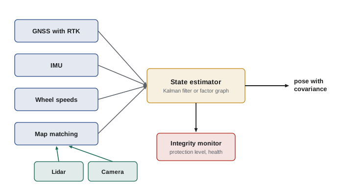
The problem for road vehicles is availability. In urban canyons between tall buildings, under bridges, in tunnels and in parking garages, satellites are blocked or their signals reflected, and RTK may lose its fix for seconds or minutes. GNSS can also be jammed or spoofed. Automated vehicles therefore never rely on GNSS alone. It provides a global reference and initial position, while inertial sensors, wheel speeds and map matching carry the estimate through outages.
Dead reckoning with inertial and wheel sensors
An inertial measurement unit, IMU, measures acceleration and angular rate. Integrating angular rate gives heading; integrating acceleration twice gives position. Wheel-speed sensors give distance travelled, and the steering angle or a yaw-rate sensor gives turning. Combining these, dead reckoning tracks motion over short periods with high rates and smooth output, but errors accumulate. A gyro bias of 10 degrees per hour, typical of automotive-grade sensors, produces a heading error of about 0.17 degrees after one minute, and wheel odometry error from tire wear, slip and pressure changes is typically a fraction of one per cent of the distance travelled.
Worked problem
Drift during a tunnel
A vehicle drives through a 1.2 km tunnel at 72 km/h with no GNSS. Its odometry has a scale error of 0.5 % and its heading drifts at 10 degrees per hour. Estimate the along-track and cross-track error at the tunnel exit if the tunnel is straight.
Show solution
- Time in tunnel: \( 1200 / 20 = 60 \) s, since 72 km/h is 20 m/s.
- Along-track error: \( 0.005 \times 1200 = 6 \) m.
- Heading drift after 60 s: \( 10/60 \approx 0.167^\circ \), growing linearly; the average heading error is half that, \( 0.083^\circ \approx 0.00145 \) rad.
- Cross-track error: \( 1200 \times 0.00145 \approx 1.7 \) m.
Answer: About 6 m along the road and 1.7 m across it, far too much for lane keeping without map matching to lane markings or tunnel walls.
Map-relative localization
The key to lane-level localization is matching what the sensors see against a prior map. Lidar-based systems compare the current point cloud with a stored map of the environment, using scan matching methods such as iterative closest point or normal distributions transform from ROB-340, or match ground reflectivity images that capture lane paint and road texture. Camera-based systems detect lane markings, signs, poles and other landmarks and match them to their mapped positions. Radar can match against maps of strong radar reflectors such as guardrails and sign gantries. The matches give corrections that are fused with GNSS, IMU and odometry in a Kalman or factor-graph estimator, as in ROB-310 and ROB-340.
# 1-D localization along a road: odometry drift corrected by occasional landmark matches
import numpy as np
rng = np.random.default_rng(7)
dt, v, T = 0.1, 20.0, 60.0                  # 20 m/s for 60 s
n = int(T / dt)
true_x = np.cumsum(np.full(n, v * dt))
odo = v * dt * (1 + 0.005) + rng.normal(0, 0.02, n)   # 0.5 % scale error + noise
x_dr = np.cumsum(odo)                        # dead reckoning only
# Kalman filter: predict with odometry, update with landmark every 10 s (sigma 0.2 m)
x, P, Q, R = 0.0, 0.01, 0.02**2 + (0.005 * v * dt)**2, 0.2**2
est = []
for k in range(n):
    x += odo[k]; P += Q
    if (k + 1) % 100 == 0:                   # landmark match
        z = true_x[k] + rng.normal(0, 0.2)
        K = P / (P + R); x += K * (z - x); P *= (1 - K)
    est.append(x)
est = np.array(est)
print(f"dead-reckoning error at end: {x_dr[-1] - true_x[-1]:6.2f} m")
print(f"filtered error at end:       {est[-1] - true_x[-1]:6.2f} m")
print(f"max filtered error: {np.max(np.abs(est - true_x)):6.2f} m")dead-reckoning error at end: 4.40 m filtered error at end: 0.23 m max filtered error: 1.36 m
High-definition maps
A high-definition, or HD, map is far richer than a navigation map. It records the three-dimensional geometry of each lane with centimetre-level accuracy, lane boundaries and their types, stop lines, crosswalks, traffic signal positions and which lanes each signal controls, signs and speed limits, curbs and road edges, and often a localization layer such as a point-cloud or reflectivity map. Semantic layers add rules: which turns are permitted from which lanes, right-of-way at intersections, school zones and their hours. The map lets the vehicle anticipate what it cannot yet see and focus perception on what has changed.
| Map layer | Contents | Used by |
|---|---|---|
| Localization layer | Point cloud, reflectivity image or landmark set | Map-relative localization |
| Lane geometry | Lane centre lines and boundaries with 3-D shape | Planning, control, prediction |
| Road furniture | Signs, signals, poles, guardrails | Localization, perception focus |
| Semantic and rules | Turn permissions, right-of-way, speed limits, school zones | Behaviour planning |
| Dynamic layer | Construction zones, closures, temporary signals | Routing and planning |
HD maps are built by driving survey vehicles with high-grade sensors through the area, processing the data offline with SLAM and bundle adjustment, then labelling lanes and rules, partly by hand and increasingly with machine learning. They are expensive to build and must be maintained, because roads change: lanes are repainted, construction zones appear, signals move. Operators detect changes by comparing what fleet vehicles see with the map and flag discrepancies for review. A vehicle that notices a mismatch between map and reality must decide whether to trust its eyes or its map, and usually treats unexplained differences as a reason for caution.
Some developers aim to reduce dependence on prior maps by building lighter maps or by having the vehicle infer lane topology online from its sensors, which makes it easier to expand to new areas. Others argue that detailed maps are an important safety layer, giving the vehicle prior knowledge that sensors alone may miss in rain or at night. Both approaches exist in deployed systems at the time of writing.
Worked problem
Map storage
An HD map stores a localization layer at about 10 MB per kilometre of road and lane and semantic layers at about 0.5 MB per kilometre. A service area contains 3,000 km of road. How much storage does the map need, and how much data does a monthly update of 5 % of the roads involve?
Show solution
- Per kilometre: \( 10 + 0.5 = 10.5 \) MB.
- Total: \( 3000 \times 10.5 = 31\,500 \) MB, about 31.5 GB.
- Monthly update of 5 %: \( 0.05 \times 31.5 \approx 1.6 \) GB per vehicle.
Answer: About 31.5 GB for the whole area and roughly 1.6 GB of updates per vehicle per month; sizes vary widely between map formats.
# Launching the open-source Autoware stack with a prior map (commands vary between releases)
source ~/autoware/install/setup.bash
ros2 launch autoware_launch autoware.launch.xml \
    map_path:=$HOME/autoware_map/campus \
    vehicle_model:=sample_vehicle sensor_model:=sample_sensor_kit
# The map folder holds a point-cloud map (pointcloud_map.pcd) for lidar localization
# and a Lanelet2 file (lanelet2_map.osm) with lane geometry and traffic rules.
# Check the localization result and its covariance:
ros2 topic echo /localization/kinematic_state --once
Open-source stacks illustrate the structure of HD maps concretely. Autoware, a ROS 2 based automated driving stack maintained by an international foundation, uses a point-cloud map for lidar localization and a Lanelet2 map that represents each lane as a pair of boundary lines with attached rules, such as speed limits, right-of-way and the traffic signals that control it. Students can open a Lanelet2 file in a text editor and see that it is a structured list of points, lines and relations, which planning code queries to find routes and stop lines.
Integrity: knowing when you are lost
Accuracy is not enough. A localization system must also know when it might be wrong. Aviation introduced the idea of integrity for satellite navigation: the system reports a protection level, a bound that the true error is guaranteed, with very high probability, not to exceed, and raises an alarm when the bound exceeds what the operation can tolerate. Automated vehicles adopt the same idea. If the estimated lateral protection level grows beyond the margin computed earlier in this lesson, because GNSS is lost, map matching fails in snow, or the map no longer matches reality, the vehicle must slow down, increase margins or reach a minimal risk condition. The localization module's honesty about its own uncertainty is a safety function.
Common mistakes
MistakeRelying on standard GNSS for lane keeping.
InsteadStandard GNSS errors are metres; lane keeping needs map matching and fusion to reach decimetres.
MistakeAssuming RTK is always available.
InsteadUrban canyons, tunnels and jamming cause outages; design for them.
MistakeIgnoring heading error.
InsteadSmall heading errors project into large lateral errors at planning distances.
MistakeTreating the HD map as permanently correct.
InsteadRoads change; detect and handle mismatches, and keep maps updated.
MistakeReporting only a best estimate.
InsteadReport uncertainty and integrity so the vehicle can react when localization degrades.
Summary and key terms
- Lane-level driving needs lateral localization within a few tens of centimetres and accurate heading.
- GNSS gives a global reference; RTK and PPP reach centimetre to decimetre accuracy in open sky but suffer outages.
- IMU and wheel odometry carry the estimate through short outages but drift over time.
- Map-relative localization matches lidar, camera or radar observations against a prior map.
- Fusion in a Kalman filter or factor graph combines all sources with their uncertainties.
- HD maps add lane geometry, rules and landmarks, and must be maintained as roads change.
- Integrity monitoring and protection levels tell the vehicle when localization can no longer be trusted.
- GNSS
- Global navigation satellite systems such as GPS, Galileo, GLONASS and BeiDou.
- RTK
- Real-time kinematic positioning using carrier phase and correction data for centimetre accuracy.
- Multipath
- Satellite signals reflecting off surfaces before reaching the antenna, causing errors.
- Dead reckoning
- Estimating position by integrating measured motion from a known start.
- Map matching
- Aligning sensor observations with a prior map to correct position.
- HD map
- A centimetre-accurate map with lane geometry, rules and localization layers.
- Scan matching
- Aligning a current point cloud with a reference cloud or map.
- Protection level
- A bound on position error that holds with a specified high probability.
- Integrity
- The ability of a navigation system to warn when its output should not be trusted.
- Change detection
- Finding differences between the map and the current environment.
Practice problems
Work each problem on paper first, then reveal the answer to check.
Lane 3.7 m, car 1.9 m: free space on each side when centred?
Show answer
0.9 m.
A 1 degree heading error projected 30 m ahead gives what lateral error?
Show answer
About 0.52 m.
Name two causes of GNSS outages for cars.
Show answer
Tunnels, urban canyons, overpasses, parking garages, jamming or spoofing.
Why does dead reckoning drift?
Show answer
Small sensor biases and scale errors accumulate when integrated.
What does a reflectivity map capture?
Show answer
Ground intensity patterns such as lane paint and road texture.
A 0.2 % odometry scale error over 2 km gives what error?
Show answer
4 m along track.
Name two HD map layers.
Show answer
Localization, lane geometry, road furniture, semantic rules or dynamic layer.
What should a vehicle do if its protection level exceeds the allowed margin?
Show answer
Slow, increase margins or reach a minimal risk condition.
Why are HD maps expensive?
Show answer
They need survey driving, processing, labelling and continuous maintenance.
What estimator types fuse localization sources?
Show answer
Kalman filters and factor graphs.
Lesson quiz · 5 questions
Score 60% or more to complete this lesson.
Create a free account to save your progress, take quizzes and earn a certificate.