
ROB-420 · Lesson 2 of 12 · 29 min
Sensors and perception for automated vehicles
An automated vehicle can only respond to what it perceives. Perception must find every relevant object around the vehicle, from cars and trucks to pedestrians, cyclists, animals and debris, estimate where each one is and how it is moving, and identify the static world: lanes, curbs, traffic signs, signals and drivable space. It must do so in daylight and darkness, in rain, fog and snow, at highway speeds and in crowded downtown streets. ROB-220 described sensors in general and ROB-330 covered computer vision. This lesson looks at the sensor suites used on road vehicles, how their coverage is designed, how their data is fused, and why weather, including a Canadian or northern US winter, remains one of the hardest problems in the field.
The automotive sensor suite
Four sensor types dominate. Cameras are cheap, high-resolution and the only sensor that reads colour, text and signals, but they measure depth only indirectly and suffer in glare and low light. Radar measures range and radial velocity directly using the Doppler effect, works in rain, fog and darkness, and sees through spray, but has coarse angular resolution and can be confused by metal objects such as manhole covers and overhead signs. Lidar fires laser pulses and measures their return time, producing precise three-dimensional point clouds day or night, but it is more expensive, has limited range on dark surfaces and degrades in heavy precipitation. Ultrasonic sensors measure short distances, a few metres, cheaply and are used for parking and low-speed manoeuvres.
| Sensor | Measures | Typical range | Strengths | Weaknesses |
|---|---|---|---|---|
| Camera | Colour images; depth by stereo or learning | Up to 200 m or more for detection with long lenses | Signals, signs, lane markings, classification, low cost | Glare, darkness, no direct depth, lens soiling |
| Radar (77 GHz) | Range, radial speed, angle | 200 to 300 m for long-range units | All weather, direct velocity, long range | Low angular resolution, clutter from metal |
| Lidar | 3-D points with intensity | 100 to 250 m depending on target reflectivity | Precise geometry, works at night | Cost, rain and snow returns, dark targets |
| Ultrasonic | Distance to nearest echo | About 0.2 to 5 m | Very cheap, parking and curbs | Short range, poor angular information |
| 4-D imaging radar | Range, speed, azimuth and elevation | Up to about 300 m | Height information, better resolution than older radar | Still coarser than lidar |
Different developers weigh these sensors differently. Most robotaxi and driverless truck programs at the time of writing (October 2026) use all three main modalities, camera, radar and lidar, so that each covers the others' weaknesses. Some driver-assistance and supervised driving systems rely mainly on cameras with neural networks that estimate depth and motion. The trade-off is between cost and simplicity on one side and redundancy and directly measured geometry on the other. For a Level 4 system that must perform its own fallback, regulators and safety assessors usually expect redundancy, so that no single sensor failure leaves the vehicle blind.
Designing coverage
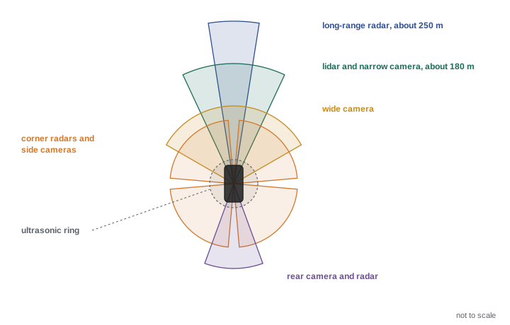
Sensor placement is planned so that the vehicle has overlapping coverage all around, with the longest range where it matters most. A car travelling forward at highway speed needs to see far ahead, perhaps 200 m or more, to detect stopped traffic in time. At an intersection it needs wide-angle views to the sides to see cross traffic. When merging or changing lanes it needs rear and side coverage to detect fast vehicles approaching from behind. When pulling away from the curb it needs near-field coverage to detect a child or a pet next to the bumper. Engineers draw coverage maps showing each sensor's field of view and range, and check that every region relevant to the ODD is covered by at least two sensors of different types.
Worked problem
How far must the vehicle see?
A truck travels at 100 km/h. Its system latency is 0.5 s and it can brake comfortably at 3 m/s². It must detect a stopped vehicle early enough to stop with a 10 m margin. What minimum detection range is needed?
Show solution
- Speed: \( v = 100 / 3.6 \approx 27.8 \) m/s.
- Distance during latency: \( 27.8 \times 0.5 \approx 13.9 \) m.
- Braking distance: \( v^2 / (2a) = 27.8^2 / 6 \approx 128.6 \) m.
- Total with margin: \( 13.9 + 128.6 + 10 \approx 153 \) m.
Answer: At least about 153 m of reliable detection range, more if the road is wet or the truck is heavily loaded.
From raw data to objects
Perception pipelines detect objects in each sensor, then associate and track them over time. Camera networks output two-dimensional or three-dimensional bounding boxes, segmentation masks and classes. Lidar networks operate on point clouds, often after converting them to a bird's-eye-view grid, and output three-dimensional boxes with headings. Radar provides detections with measured radial velocity. A tracker, usually built on the Kalman and multi-target tracking ideas from ROB-310, associates detections across frames, estimates each object's position, velocity, heading and size, and keeps track identities stable. The output is a list of tracked objects with uncertainty, plus static map elements such as lane boundaries and traffic light states.
Many modern stacks fuse sensor data inside the neural network rather than after detection. In a bird's-eye-view, or BEV, architecture, features from all cameras are projected into a common top-down grid around the vehicle, often combined with lidar and radar features, and a single network outputs objects, lanes and occupancy. Occupancy networks go further and predict, for every cell in a three-dimensional grid around the vehicle, whether it is occupied and how it is moving, which helps with unusual objects that do not fit any trained class, such as a fallen ladder or an overturned shopping cart.
| Fusion level | What is combined | Advantage | Disadvantage |
|---|---|---|---|
| Early (raw data) | Pixels and points before detection | Uses all information | Needs precise calibration and synchronization; large networks |
| Mid (features) | Learned features, for example in a BEV grid | Strong performance, handles occlusion well | Harder to diagnose which sensor contributed |
| Late (objects) | Detections or tracks from each sensor | Modular, each sensor tested separately | Information discarded early; weak cues lost |
Fusing measurements with uncertainty
Whatever the architecture, the principle of fusion is the same as in ROB-310: combine measurements in proportion to how much you trust them. If a radar measures an object's range with a standard deviation of 0.5 m and a camera-based estimate has a standard deviation of 2 m, the fused estimate should lean heavily on the radar. For independent Gaussian measurements of the same quantity, the minimum-variance combination weights each measurement by the inverse of its variance.
# Inverse-variance fusion of radar and camera range estimates (toy example)
import numpy as np
rng = np.random.default_rng(42)
true_range = 48.0
sig_radar, sig_cam = 0.5, 2.0
radar = true_range + rng.normal(0, sig_radar, 1000)
cam = true_range + rng.normal(0, sig_cam, 1000)
w_r, w_c = 1 / sig_radar**2, 1 / sig_cam**2
fused = (w_r * radar + w_c * cam) / (w_r + w_c)
for name, est in (("radar", radar), ("camera", cam), ("fused", fused)):
    print(f"{name:6s} mean {est.mean():6.2f} m  std {est.std():5.2f} m")
print(f"predicted fused std {(w_r + w_c) ** -0.5:5.2f} m")radar mean 47.99 m std 0.49 m camera mean 47.84 m std 2.03 m fused mean 47.98 m std 0.48 m predicted fused std 0.49 m
Worked problem
Fusing two velocity estimates
Radar measures a car's closing speed as 8.0 m/s with standard deviation 0.2 m/s. A camera tracker estimates 9.0 m/s with standard deviation 1.0 m/s. What is the fused estimate and its standard deviation?
Show solution
- Weights: \( 1/0.2^2 = 25 \) and \( 1/1.0^2 = 1 \).
- Fused value: \( (25 \times 8.0 + 1 \times 9.0)/26 = 209/26 \approx 8.04 \) m/s.
- Fused standard deviation: \( (25 + 1)^{-1/2} \approx 0.196 \) m/s.
Answer: About 8.04 m/s with standard deviation about 0.20 m/s; the result leans almost entirely on the more precise radar.
Weather and the northern winter
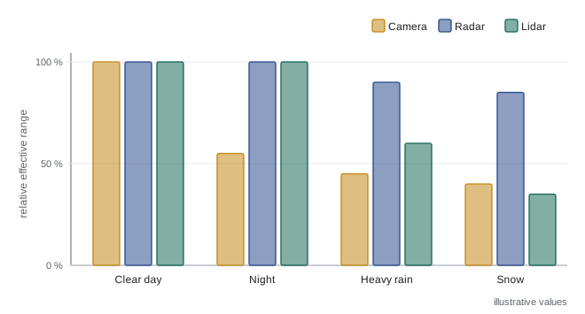
Weather affects every sensor. Rain and snow create false lidar returns and scatter laser light, so effective range falls; wet roads reflect lights and blur lane markings for cameras; spray from trucks blinds sensors at highway speed. Fog attenuates lidar and cameras strongly while radar continues to work. Low sun near sunrise and sunset dazzles cameras, a particular problem in winter at northern latitudes when the sun stays low all day. Snow covers lane markings and curbs, changes the shape of the road edge and builds up on sensor windows, while salt spray dries into an opaque film.
Developers respond in several ways. Hardware measures include heated and wiped sensor windows, air knives and washer jets, and placing sensors where they stay cleaner. Software measures include filtering precipitation noise from point clouds, training networks on winter data, relying more on radar and on maps when markings are hidden, and monitoring sensor health so that the system knows when its perception is degraded. Finally, the ODD can exclude conditions the system cannot handle, so that the vehicle reaches a minimal risk condition or does not start a trip when heavy snow is forecast. Canadian research groups, test tracks and university teams have contributed substantially to winter driving datasets and testing, and many operators that serve northern cities treat snow as one of the last conditions to add to the ODD.
Worked problem
Range loss in snow
A lidar detects a dark car reliably at 150 m in clear weather. Under moderate snow, a simple model reduces effective range by a factor \( e^{-\alpha d} \) on the round trip, so the received signal falls by \( e^{-2\alpha d} \). If the detection threshold is unchanged and \( \alpha = 0.004 \) per metre, roughly how far can the lidar now see if signal also falls with \( 1/d^2 \)?
Show solution
- In clear weather, signal at 150 m is proportional to \( 1/150^2 \).
- Find \( d \) where \( e^{-0.008 d}/d^2 = 1/150^2 \).
- Try \( d = 100 \): \( e^{-0.8}/10\,000 \approx 4.49 \times 10^{-5} \), slightly above \( 1/22\,500 \approx 4.44 \times 10^{-5} \).
- Try \( d = 101 \): \( e^{-0.808}/10\,201 \approx 4.37 \times 10^{-5} \), slightly below the threshold.
Answer: About 100 m, a one-third reduction, which would force a lower speed for the same stopping margin.
Measuring perception performance
Perception is evaluated with metrics such as precision and recall for detection, mean average precision over intersection-over-union thresholds, tracking metrics such as identity switches, and position and velocity errors. For safety, aggregate averages are not enough. What matters is performance on the objects and situations that could cause harm: a pedestrian partly hidden by a parked van, a cyclist at night, a motorcycle between lanes. Developers therefore define safety-relevant metrics, such as the time between an object becoming visible and the first stable track, or the maximum distance at which a child-sized pedestrian is reliably detected, and track them across releases.
Common mistakes
MistakeAssuming one sensor type can handle every condition.
InsteadEach modality has weaknesses; Level 4 systems normally rely on complementary, redundant sensors.
MistakeAveraging sensor measurements equally.
InsteadWeight each measurement by its precision, as in inverse-variance fusion and Kalman filtering.
MistakeDesigning coverage only for the forward direction.
InsteadIntersections, merges and curbside stops need side, rear and near-field coverage.
MistakeIgnoring sensor cleaning and blockage.
InsteadSnow, salt and mud blind sensors; plan cleaning and monitor sensor health.
MistakeJudging perception by average accuracy alone.
InsteadTrack safety-relevant metrics for vulnerable road users and hard cases.
Summary and key terms
- Automated vehicles use cameras, radar, lidar and ultrasonic sensors with complementary strengths.
- Coverage maps ensure long forward range and overlapping coverage around the vehicle.
- Required detection range follows from speed, latency and braking capability.
- Perception detects and tracks objects, lanes, signals and free space, often with bird's-eye-view networks.
- Fusion weights measurements by their precision; fused estimates are more precise than any single sensor.
- Rain, fog, snow, glare and dirty sensors reduce performance, and winter is a major challenge.
- Perception must be judged on safety-relevant metrics, not only on averages.
- Radar
- A sensor that measures range and radial velocity with radio waves.
- Lidar
- A sensor that measures distance by timing laser pulses, producing point clouds.
- Coverage map
- A diagram of each sensor's field of view and range around the vehicle.
- Bird's-eye view (BEV)
- A top-down grid representation into which sensor features are projected.
- Occupancy network
- A model predicting which cells of a 3-D grid are occupied and how they move.
- Sensor fusion
- Combining data from several sensors to obtain a better estimate.
- Inverse-variance weighting
- Combining estimates with weights proportional to the inverse of their variances.
- Track
- An object's estimated state maintained over time by a tracker.
- Sensor degradation
- Reduced performance caused by weather, dirt, damage or ageing.
- Vulnerable road user
- A pedestrian, cyclist or other road user without a vehicle's protection.
Practice problems
Work each problem on paper first, then reveal the answer to check.
Which sensor measures radial velocity directly?
Show answer
Radar, using the Doppler effect.
Which sensor reads traffic signal colour?
Show answer
The camera.
At 25 m/s with 0.4 s latency and 4 m/s² braking, what range is needed to stop?
Show answer
About 10 + 78 = 88 m, plus any margin.
Two range estimates have standard deviations 1 m and 1 m. What is the fused standard deviation?
Show answer
About 0.71 m.
Why are winter conditions hard for cameras?
Show answer
Snow hides markings, low sun dazzles, and spray or salt soils lenses.
What is late fusion?
Show answer
Combining detections or tracks produced separately by each sensor.
Give one hardware measure against sensor soiling.
Show answer
Heaters, wipers, washer jets or air knives.
Why do occupancy networks help with unusual objects?
Show answer
They predict occupied space without needing a known object class.
What metric might capture the danger of a late detection?
Show answer
Time from an object becoming visible to a stable track.
Why do Level 4 systems usually carry redundant sensors?
Show answer
So that no single sensor failure leaves the system blind during fallback.
Lesson quiz · 5 questions
Score 60% or more to complete this lesson.
Create a free account to save your progress, take quizzes and earn a certificate.