
ROB-350 · Lesson 5 of 12 · 30 min
Grid and lattice planning
Most mobile robots plan on grids. The robot's map, built by the SLAM methods of ROB-340, is already an occupancy grid; turning it into a planning graph needs only a decision about which cells are traversable and what each step costs. Grid planning is resolution complete, simple to implement, fast in two dimensions and easy to update as the map changes, which is why it dominates indoor navigation. Its weaknesses are equally well known: paths constrained to grid directions, which zigzag and hug walls, and no notion of what motions the robot can actually execute. This lesson covers how to build a good planning grid from a map, how to get smoother paths from it, and how state lattices and Hybrid A* extend grid search to robots, such as cars, that cannot turn on the spot.
From occupancy grid to cost map
An occupancy grid stores, for each cell, the probability that it is occupied. A planner needs a cost per cell instead. The usual construction, used in ROS 2 Nav2's costmap layers, marks cells above an occupancy threshold as lethal obstacles, then inflates them. Every cell within the robot's inscribed radius of an obstacle is marked as an inscribed obstacle: if the robot's centre were there, some part of it would certainly collide. Beyond that, cost decays with distance out to an inflation radius, giving the planner a reason to stay away from obstacles when it has room. Unknown cells get a separate cost chosen by policy. A common decay is exponential:
where d is the distance to the nearest obstacle, \( r_{\text{in}} \) is the inscribed radius and α sets how fast the cost falls. The distance to the nearest obstacle for every cell is computed in one pass with a brushfire (breadth-first) search from the obstacles or with a distance transform, so building the cost map is linear in the number of cells. Layered cost maps combine several sources: a static layer from the saved map, an obstacle layer from live sensor data, and inflation on top. The navigation stack itself, with its layers and plugins, is covered in ROB-340 lesson 11; here the focus is on what the planner does with the costs.
Worked problem
Inflation costs
A cost map uses \( c_{\text{inscribed}} = 253 \), inscribed radius 0.30 m, inflation radius 0.90 m and \( \alpha = 5 \) per metre. What cost do cells at 0.40 m, 0.60 m and 1.00 m from the nearest obstacle receive?
Show solution
- At 0.40 m: \( 253\,e^{-5(0.10)} = 253 \times 0.607 \approx 153 \).
- At 0.60 m: \( 253\,e^{-5(0.30)} = 253 \times 0.223 \approx 56 \).
- At 1.00 m: beyond the inflation radius, so cost 0 (free).
Answer: About 153, 56 and 0. A smaller α spreads the cost further and pushes paths toward the middle of corridors; a larger α lets the robot pass closer to obstacles.
Grid resolution and connectivity
Choosing the cell size is a trade-off. Smaller cells represent narrow gaps and precise obstacle shapes but multiply the number of nodes by four each time the size halves, and they make the map noisier. Indoor robots commonly use 5 cm cells; outdoor vehicles 10 to 50 cm. Connectivity matters too. On a 4-connected grid, the shortest path between two points is a staircase whose length can exceed the straight-line distance by up to 41 per cent. On an 8-connected grid the worst case is about 8 per cent, at an angle of 22.5°. A 16-connected grid, adding moves like two cells across and one up, cuts this to about 3 per cent. Even then, grid paths change direction only at multiples of the allowed angles, and they tend to graze the corners of obstacles where the grid is tight.
Worked problem
Worst-case grid path lengths
The straight-line distance between two cells is 10 m along a direction 22.5° from the x-axis. How long is the shortest path on 4-connected and 8-connected grids, ignoring obstacles?
Show solution
- Components: \( \Delta x = 10\cos 22.5^{\circ} = 9.24 \) m, \( \Delta y = 10\sin 22.5^{\circ} = 3.83 \) m.
- 4-connected: \( \Delta x + \Delta y = 13.07 \) m, 31 per cent longer.
- 8-connected: \( \max + (\sqrt{2} - 1)\min = 9.24 + 0.414 \times 3.83 = 10.82 \) m, 8.2 per cent longer.
Answer: 13.07 m and 10.82 m. The 8-connected grid is much closer, but still produces a path with an unnecessary bend, which post-processing or any-angle search can remove.
Smoother paths: post-processing and any-angle search
Two families of techniques remove grid artefacts. Post-processing takes the grid path and shortens it. The simplest method is line-of-sight shortcutting: walk along the path and, whenever a later waypoint is directly visible from the current one, delete the waypoints in between. The result is a sequence of straight segments, much like a visibility-graph path. Smoothing with splines or a gradient method (lesson 9) then rounds the corners. Any-angle search algorithms instead build line of sight into the search. Theta* (Nash, Daniel, Koenig and Felner, 2007) is A* in which, when a node is relaxed, it checks whether the node's parent's parent can see the neighbour directly; if so, it links them with a straight segment. Theta* paths are close to true shortest paths and need little smoothing. Field D* applies a similar idea to incremental replanning by interpolating costs along cell edges.
import math
# Line-of-sight shortcutting of an 8-connected grid path (rows, cols), with a free 10 x 10 area and one blocked cell
blocked = {(3, 4), (4, 4), (5, 4)}
path = [(0,0),(1,1),(2,2),(2,3),(1,4),(1,5),(2,6),(3,7),(4,8),(5,9),(6,9),(7,9)]
def visible(a, b, steps=50):
    for k in range(steps + 1):
        t = k / steps
        r, c = a[0] + t * (b[0] - a[0]), a[1] + t * (b[1] - a[1])
        if (round(r), round(c)) in blocked: return False
    return True
def length(p): return sum(math.dist(p[i], p[i + 1]) for i in range(len(p) - 1))
short = [path[0]]; i = 0
while i < len(path) - 1:
    j = len(path) - 1
    while j > i + 1 and not visible(path[i], path[j]): j -= 1
    short.append(path[j]); i = j
print("grid path: %d waypoints, length %.2f cells" % (len(path), length(path)))
print("shortcut:  %d waypoints, length %.2f cells" % (len(short), length(short)))
print("kept:", short)grid path: 12 waypoints, length 13.90 cells shortcut: 3 waypoints, length 12.30 cells kept: [(0, 0), (5, 9), (7, 9)]
State lattices for car-like robots
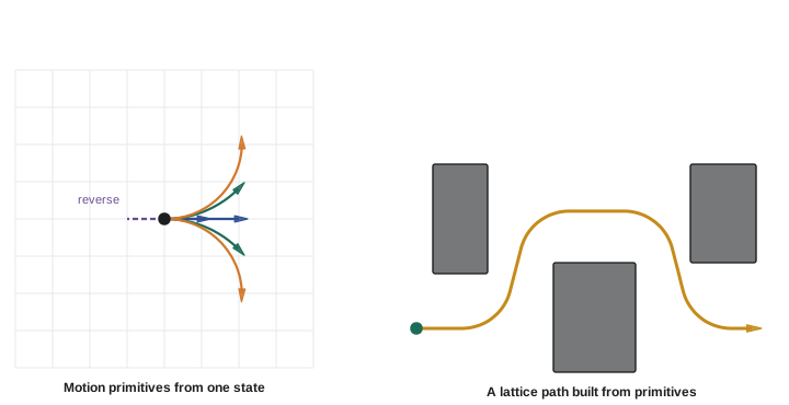
A grid over (x, y) cannot represent a robot that must respect its heading and turning radius. Adding a heading dimension gives a three-dimensional grid over (x, y, θ), but joining neighbouring cells with straight steps still ignores the turning constraint. State lattices, developed by Pivtoraiko, Knepper and Kelly around 2009, solve this by building the graph from motion primitives: short, dynamically feasible trajectories that start and end exactly on lattice states. For example, with headings discretized into 16 directions, each heading has a set of primitives that move forward a few cells and end at the same or an adjacent heading, plus reverse and turning primitives if the robot allows them. Because every primitive is feasible and they join exactly at lattice states, any path through the lattice is executable. The primitives are computed offline, usually by solving a small boundary-value problem, together with the cells they sweep, so collision checking a primitive at search time means checking a precomputed footprint.
Worked problem
Sizing a lattice
A lattice uses 10 cm cells on a 60 m by 40 m warehouse map and 16 headings, with 7 primitives per heading. How many states and edges does the full lattice have?
Show solution
- Cells: \( (60/0.1) \times (40/0.1) = 600 \times 400 = 240{,}000 \).
- States: \( 240{,}000 \times 16 = 3.84 \times 10^{6} \).
- Edges: \( 3.84 \times 10^{6} \times 7 \approx 2.7 \times 10^{7} \).
Answer: About 3.8 million states and 27 million edges. A* with a good heuristic expands only a small fraction of these, but the heuristic now matters much more than on a 2-D grid.
Hybrid A*
Hybrid A*, used by Stanford's Junior in the 2007 DARPA Urban Challenge and described by Dolgov, Thrun, Montemerlo and Diebel, combines a grid with continuous states. Each search node holds a continuous pose (x, y, θ), but nodes are associated with discretized cells, and only one node is kept per cell (the cheapest). Expanding a node applies a few steering commands, such as full left, straight and full right, forward and in reverse, for a fixed arc length, producing new continuous poses. Because states are continuous, paths are drivable without lattice alignment, at the cost of losing resolution completeness: pruning by cell may discard a node that was needed. Two heuristics are combined, taking the maximum: a nonholonomic heuristic that ignores obstacles (the Reeds-Shepp distance) and a holonomic heuristic that ignores turning (a 2-D Dijkstra distance on the obstacle map). At regular intervals, the planner also tries an analytic expansion, connecting the current node directly to the goal with a Reeds-Shepp curve; if that curve is collision-free, the search ends early with an exact final approach. The resulting path is then smoothed by optimization. Hybrid A* remains a standard choice for parking and for car-like robots in unstructured spaces.
Worked problem
Expansion step for Hybrid A*
A car with wheelbase 2.7 m expands a node at (10.0, 5.0) m, heading 0°, by driving 1.5 m forward with steering angle 25°. Using the bicycle model, what is the new heading and approximate position?
Show solution
- Turning radius: \( R = L/\tan\delta = 2.7/\tan 25^{\circ} = 2.7/0.466 = 5.79 \) m.
- Heading change: \( \Delta\theta = s/R = 1.5/5.79 = 0.259 \) rad = 14.8°.
- Position on the arc: \( x = 10.0 + R\sin\Delta\theta = 10.0 + 5.79 \times 0.256 = 11.48 \) m; \( y = 5.0 + R(1 - \cos\Delta\theta) = 5.0 + 5.79 \times 0.033 = 5.19 \) m.
Answer: About (11.48, 5.19) m with heading 14.8°. This pose is kept as continuous values and filed under the cell containing it.
| Method | State | Feasible paths? | Guarantee | Typical use |
|---|---|---|---|---|
| 2-D grid A* | (x, y) | No turning constraint | Resolution complete, optimal on grid | Indoor differential-drive robots |
| Theta* / any-angle | (x, y) | No turning constraint | Near-shortest | Smooth global paths |
| State lattice | (x, y, θ) discretized | Yes, by construction | Resolution complete, optimal on lattice | Cars, tugs, forklifts |
| Hybrid A* | Continuous (x, y, θ), cell pruning | Yes | Not resolution complete | Parking, unstructured driving |
Common mistakes
MistakePlanning on the raw occupancy grid without inflation
InsteadInflate by at least the inscribed radius so the centre path keeps the body clear.
MistakeSetting the inflation cost so high and wide that corridors close
InsteadTune α and the inflation radius so narrow passages stay traversable.
MistakeSending a raw 8-connected grid path straight to the controller
InsteadShortcut and smooth it, or use an any-angle planner.
MistakeUsing a 2-D grid planner for a car-like robot and hoping the controller copes
InsteadUse a lattice or Hybrid A* so the path respects the turning radius.
MistakeUsing Euclidean distance as the only heuristic for a lattice planner
InsteadCombine a turning-aware heuristic with an obstacle-aware 2-D heuristic.
Summary and key terms
- Grid planners turn an occupancy grid into a cost map with lethal, inscribed and inflated costs.
- Inflation is computed with a distance transform and encourages clearance without forbidding narrow passages.
- Cell size and connectivity trade accuracy against speed; 8-connected grid paths are up to about 8 per cent too long.
- Line-of-sight shortcutting and any-angle search such as Theta* remove grid artefacts.
- State lattices build the graph from precomputed feasible motion primitives, so every path can be driven.
- Hybrid A* keeps continuous poses filed by cell, expands with steering arcs and uses analytic Reeds-Shepp expansions.
- Good heuristics, combining turning and obstacles, are essential for planners in (x, y, θ).
- Cost map
- A grid storing a traversal cost for each cell.
- Lethal cost
- The cost marking a cell occupied by an obstacle.
- Inflation
- Raising the cost of cells near obstacles.
- Distance transform
- Computing each cell's distance to the nearest obstacle.
- Shortcutting
- Removing waypoints that can be skipped by a straight, collision-free segment.
- Any-angle search
- Grid search that allows straight segments in any direction.
- Theta*
- An any-angle variant of A* that links grandparents by line of sight.
- Motion primitive
- A short feasible trajectory between lattice states.
- State lattice
- A graph of discretized states joined by motion primitives.
- Hybrid A*
- A* over continuous poses with cell-based pruning, for car-like robots.
Practice problems
Work each problem on paper first, then reveal the answer to check.
What cells are marked as inscribed obstacles?
Show answer
Cells within the inscribed radius of an obstacle.
How is each cell's distance to obstacles computed efficiently?
Show answer
With a brushfire search or distance transform.
Worst-case path stretch on an 8-connected grid?
Show answer
About 8 per cent.
What does halving the cell size do to the number of 2-D cells?
Show answer
Multiplies it by four.
How does Theta* differ from A*?
Show answer
It links a node to its parent's parent when there is line of sight.
What guarantees a lattice path is drivable?
Show answer
Every edge is a precomputed feasible primitive.
Turning radius for wheelbase 3.0 m and steering 30°?
Show answer
3.0 / tan 30° ≈ 5.2 m.
Name the two heuristics in Hybrid A*.
Show answer
Reeds-Shepp distance and 2-D Dijkstra distance.
What is an analytic expansion?
Show answer
Connecting directly to the goal with a Reeds-Shepp curve.
Which guarantee does Hybrid A* give up?
Show answer
Resolution completeness.
Lesson quiz · 5 questions
Score 60% or more to complete this lesson.
Create a free account to save your progress, take quizzes and earn a certificate.