
ROB-350 · Lesson 12 of 12 · 28 min
Capstone: a planner for a warehouse mobile manipulator
This capstone brings the course together in a single design. A company is deploying mobile manipulators in a fulfilment warehouse: a differential-drive base, 0.7 m by 0.6 m, carrying a 7-joint arm with a suction gripper. Each robot drives to a shelf, picks totes or items from shelf bays and drops them into a bin on its back, then drives to a packing station. Aisles are 1.2 m wide, with people and other robots sharing them. The task is to choose planners for each part of the job, justify the choices with the methods of lessons 1 to 11, define how the system will be benchmarked, and decide what to do when planning fails. As in the capstones of ROB-310 and ROB-340, the result is a design document with numbers, not a single algorithm.
Requirements
Good planning systems start from measurable requirements. The operations team and safety engineers agreed the following for this deployment. They mix performance (planning time, path quality), reliability (success rate) and safety (clearance, behaviour near people), and they make explicit what happens when the planner cannot find a solution.
| Requirement | Target | Why it matters |
|---|---|---|
| Base global planning time | ≤ 100 ms (95th percentile) on a 120 m × 60 m map | Replanning at 1 Hz must not delay the robot |
| Base local control rate | ≥ 20 Hz | React to people stepping into the aisle |
| Base clearance | ≥ 0.15 m from static obstacles, ≥ 0.5 m from people | Safety margin budget and comfort |
| Arm planning time | ≤ 0.5 s (95th percentile) per pick motion | Picks per hour target |
| Arm planning success | ≥ 99.5 % on the benchmark pick set | Each failure costs a human intervention |
| Path quality | Arm joint-path length within 1.3 × the best found offline | Cycle time and predictability |
| Failure behaviour | Report failure within 1 s, with a reason | Lets the fleet manager reassign or reposition |
The base: global and local planning
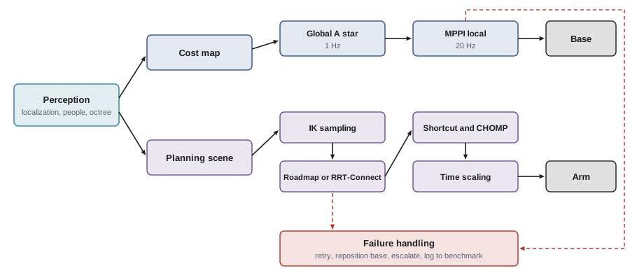
The base is a differential-drive robot, so it can turn on the spot and a path in (x, y) is executable if the footprint fits (lesson 10). Its configuration space is effectively three-dimensional only in tight spots. The map is a static occupancy grid from the SLAM system of ROB-340, at 5 cm resolution, which gives \( 2400 \times 1200 = 2.88 \times 10^{6} \) cells. A 2-D A* on an inflated cost map is the natural global planner (lessons 4 and 5): the inflation uses the 0.30 m inscribed radius as the lethal band and an exponential decay out to 0.9 m so that paths prefer the middle of aisles. Because the footprint is rectangular with a 0.46 m circumscribed radius and aisles are 1.2 m wide, the robot can always rotate in an aisle, so footprint checks are needed only at shelf bays and doorways, where the local planner checks the full rectangle. With the octile heuristic, a cross-warehouse query expands a few hundred thousand cells in the worst case, comfortably within 100 ms in compiled code; weighted A* with w = 1.5 is held in reserve if profiling shows otherwise.
Locally, an MPPI controller (lesson 11) follows the global path at 20 Hz, using a 2 s horizon and the robot's acceleration limits, with people tracked by the perception system and predicted at constant velocity. People get a 0.5 m social margin, inflated further by their prediction uncertainty (lesson 11, chance constraints). If the local controller cannot make progress for 3 s, for example because an aisle is blocked, it reports to the global planner, which marks the blockage in a temporary layer and replans around it.
Worked problem
Global planner budget
Profiling shows that A* on this map expands about 450,000 nodes for the longest routes, at 180 ns per expansion including neighbour generation and cost-map lookups. Does it meet the 100 ms target, and what weight would weighted A* need to halve the expansions if experiments show expansions fall roughly as \( 1/w^{1.5} \)?
Show solution
- Time: \( 450{,}000 \times 180 \) ns = 81 ms, within 100 ms but with little margin.
- Halving expansions: \( w^{1.5} = 2 \), so \( w = 2^{2/3} = 1.59 \).
- The worst-case path cost would then be at most 1.59 times optimal, though typically within a few per cent.
Answer: About 81 ms, so it meets the target. A weight of about 1.6 would halve the work if more margin is needed, at a bounded cost in path quality.
The arm: picking motions
The arm has seven joints, so grids are out (lesson 1) and the pick motions are planned with a sampling planner followed by optimization, using MoveIt 2 (lesson 11). Each pick is a sequence: a free-space transfer from the stowed configuration to a pre-pick pose 10 cm in front of the item; a straight Cartesian approach to the suction point; attaching the item to the robot model; a straight retreat; and a free-space transfer to the drop pose above the onboard bin. The free-space transfers use RRT-Connect (lesson 7) with a 0.5 s budget, followed by shortcutting and a short CHOMP pass (lesson 9) to smooth the path while keeping 3 cm of clearance from shelf edges. The collision model uses capsules for the arm links and convex hulls for the shelf and bin fixtures (lesson 8), plus an octree from the wrist camera for unexpected clutter in the bay. The padding budget follows lesson 8: encoder and calibration error, tracking error, camera error and base localization error at the shelf, combined by root sum of squares.
Because the shelf bays are fixed, the system can also learn. A PRM (lesson 6) built offline for each bay type gives a library of collision-free paths between common pre-pick and drop configurations; at run time the planner first tries a roadmap query and falls back to RRT-Connect only when the scene differs, for example when the octree shows an unexpected object. This multi-query reuse cuts the median planning time and makes motions more repeatable, which operators value.
Worked problem
Margin budget at the shelf
Error sources at the gripper when reaching into a bay: base localization at the shelf ±12 mm (after docking with markers), arm calibration ±3 mm, tracking ±4 mm, shelf position in the map ±6 mm. Using root-sum-square and a factor of 1.5, what padding should the planner use, and does a 60 mm gap between the item and the bay ceiling leave room for the 40 mm suction cup?
Show solution
- Root sum of squares: \( \sqrt{144 + 9 + 16 + 36} = \sqrt{205} = 14.3 \) mm.
- With factor 1.5: about 21 mm.
- Space needed: cup 40 mm plus 21 mm padding = 61 mm, slightly more than the 60 mm gap.
Answer: About 21 mm of padding, which leaves the 60 mm gap just too tight. Options are better base localization at the shelf (halving the 12 mm term brings the padding to about 13 mm), a smaller cup, or approaching from a different angle.
Benchmarking
Planners must be compared on representative problems, not on a single demonstration. The team builds a benchmark of 2,000 base routes sampled from real order data and 5,000 pick problems taken from recorded shelf scans, including hard cases: items at the back of top shelves, bays with clutter, and drops when the onboard bin is nearly full. Each planner configuration is run on every problem with several random seeds, recording success, planning time, path length (or joint-path length), minimum clearance and number of collision checks. Results are reported as distributions, with medians and 95th percentiles, because averages hide the slow outliers that stall operations. OMPL's benchmarking tools and MoveIt's benchmark package support exactly this workflow, and the results drive configuration choices such as RRT-Connect's range parameter, the shortcutting budget and whether to enable the roadmap library.
import numpy as np, heapq, math
rng = np.random.default_rng(12)
# Benchmark a grid A* and a basic RRT on 40 random warehouse-like maps (rack rows with gaps); report success and path length ratio
def make_map():
    g = np.zeros((40, 60), bool)
    for r in range(5, 36, 6):
        g[r:r + 2, 4:56] = True
        for _ in range(3):
            c = rng.integers(8, 52); g[r:r + 2, c:c + 3] = False
    return g
def astar(g, s, t):
    D = [(dr, dc, math.hypot(dr, dc)) for dr in (-1, 0, 1) for dc in (-1, 0, 1) if dr or dc]
    h = lambda n: math.hypot(n[0] - t[0], n[1] - t[1])
    best = {s: 0.0}; pq = [(h(s), s)]; done = set()
    while pq:
        f, u = heapq.heappop(pq)
        if u in done: continue
        if u == t: return best[u]
        done.add(u)
        for dr, dc, c in D:
            v = (u[0] + dr, u[1] + dc)
            if 0 <= v[0] < 40 and 0 <= v[1] < 60 and not g[v] and best[u] + c < best.get(v, 1e9):
                best[v] = best[u] + c; heapq.heappush(pq, (best[v] + h(v), v))
    return None
def rrt(g, s, t, iters=800, eta=2.0):        # fixed budget of 800 iterations
    free = lambda p: 0 <= p[0] < 40 and 0 <= p[1] < 60 and not g[int(p[0]), int(p[1])]
    seg = lambda a, b: all(free(a + (b - a) * k) for k in np.linspace(0, 1, int(np.linalg.norm(b - a) / 0.25) + 2))
    N = [np.array(s, float)]; P = [-1]; T = np.array(t, float)
    for _ in range(iters):
        q = T if rng.random() < 0.1 else rng.uniform([0, 0], [40, 60])
        i = int(np.argmin([np.sum((n - q) ** 2) for n in N])); d = q - N[i]; L = np.linalg.norm(d)
        new = q if L <= eta else N[i] + eta * d / L
        if seg(N[i], new):
            N.append(new); P.append(i)
            if np.linalg.norm(new - T) < eta and seg(new, T):
                k, cost = len(N) - 1, np.linalg.norm(new - T)
                while P[k] >= 0: cost += np.linalg.norm(N[k] - N[P[k]]); k = P[k]
                return cost
    return None
ok_a = ok_r = 0; ratios = []
for _ in range(40):
    g = make_map(); s, t = (1, 1), (38, 58)
    a = astar(g, s, t); r = rrt(g, s, t)
    ok_a += a is not None; ok_r += r is not None
    if a and r: ratios.append(r / a)
print("A* solved %d of 40, RRT solved %d of 40" % (ok_a, ok_r))
print("RRT path length / A* path length: median %.2f, 90th percentile %.2f" % (np.median(ratios), np.percentile(ratios, 90)))A* solved 40 of 40, RRT solved 28 of 40 RRT path length / A* path length: median 1.22, 90th percentile 1.31
Worked problem
Is 99.5 per cent success met?
On the 5,000-problem pick benchmark, the arm configuration succeeds on 4,981 problems. What is the success rate and an approximate 95 per cent lower confidence bound, and does it meet the 99.5 per cent target?
Show solution
- Success rate: \( 4981/5000 = 99.62 \) per cent; failures 19.
- Standard error: \( \sqrt{0.9962 \times 0.0038/5000} = 0.00087 \), about 0.087 per cent.
- Lower bound: \( 99.62 - 1.645 \times 0.087 = 99.48 \) per cent (one-sided 95 per cent).
Answer: The measured rate of 99.62 per cent exceeds the target, but the lower confidence bound of about 99.48 per cent does not quite. The team should study the 19 failures, which usually cluster in a few bay types, before declaring the requirement met.
Failure handling and fallbacks
No planner succeeds every time, so the design specifies what happens when one fails. For the base, the global planner reports 'no path' with the blocking region if A* exhausts the reachable cells, and the fleet manager reroutes or alerts staff; the local controller stops and waits if a person blocks the way, then asks for a replan. For the arm, a failed RRT-Connect attempt is retried with a different IK solution and seed, then with a larger time budget, then with the base repositioned 10 cm to give a better reach; after three attempts the item is flagged for human picking. Every failure is logged with the planning scene, so it can be added to the benchmark. Over time, this loop, deploy, log failures, add them to the benchmark, tune, is what drives success rates from the high 90s toward the 99.5 per cent target.
| Component | Choice | Lesson | Main reason |
|---|---|---|---|
| Base global planner | A* on inflated cost map (weighted A* in reserve) | 4, 5 | Low-dimensional, fast, optimal on grid |
| Base local planner | MPPI at 20 Hz with people prediction | 11 | Reacts to moving people within dynamic limits |
| Arm free-space planner | Roadmap library, RRT-Connect fallback | 6, 7 | High-dimensional; reuse in fixed bays |
| Arm path smoothing | Shortcutting plus CHOMP | 7, 9 | Shorter, smoother, predictable motions |
| Approach and retreat | Cartesian straight-line paths | 11 | Predictable motion near shelves |
| Collision model | Capsules, convex hulls, wrist-camera octree | 8 | Fast checks with distance information |
| Failure handling | Retries, repositioning, human escalation, logging | 12 | Bounded failure time and continuous improvement |
Common mistakes
MistakeChoosing a planner before writing measurable requirements
InsteadFix timing, success, clearance and failure targets first, then choose methods to meet them.
MistakeBenchmarking on a handful of hand-picked problems
InsteadUse hundreds or thousands of realistic problems, several seeds, and report distributions.
MistakeReporting only mean planning time
InsteadReport medians and 95th percentiles; slow outliers stall operations.
MistakeLeaving failure behaviour unspecified
InsteadDefine retries, fallbacks, time limits and escalation.
MistakeTreating the benchmark as fixed
InsteadAdd logged field failures to it so it reflects real problems.
Summary and key terms
- A planning system starts from measurable requirements for time, success, quality, clearance and failure behaviour.
- The differential-drive base uses A* on an inflated cost map globally and an MPPI controller locally.
- The 7-joint arm uses a roadmap library with RRT-Connect fallback, shortcutting and CHOMP, with Cartesian approaches.
- Collision models and padding follow a margin budget combining localization, calibration, tracking and map errors.
- Benchmarks of thousands of realistic problems with distributions and confidence bounds decide configurations.
- Failures are bounded in time, handled by retries and fallbacks, and logged back into the benchmark.
- The design draws on every lesson: C-space, search, sampling, collision checking, optimization, nonholonomic and dynamic planning.
- Requirement
- A measurable target the planning system must meet.
- Benchmark
- A fixed set of representative problems used to compare planners.
- 95th percentile
- The value below which 95 per cent of measurements fall.
- Roadmap library
- Precomputed collision-free paths reused for repeated tasks.
- Fallback
- An alternative strategy used when the primary planner fails.
- Pre-pick pose
- A pose in front of an item from which the gripper approaches in a straight line.
- Social margin
- Extra clearance kept from people for comfort and safety.
- Confidence bound
- A limit that a true rate exceeds with stated confidence.
- Escalation
- Handing a task to a human or higher-level system after repeated failure.
- Failure logging
- Recording failed planning problems for analysis and benchmarking.
Practice problems
Work each problem on paper first, then reveal the answer to check.
Why is a 2-D grid planner suitable for the base?
Show answer
It is a differential-drive robot that can turn on the spot in 1.2 m aisles.
Why not a grid for the arm?
Show answer
Seven dimensions make grids far too large.
How many cells in a 120 m by 60 m map at 5 cm?
Show answer
2.88 million.
What does the roadmap library speed up?
Show answer
Repeated picks in fixed bay types.
Root-sum-square of 10, 5 and 5 mm?
Show answer
About 12.2 mm.
Why report the 95th percentile of planning time?
Show answer
Slow outliers matter more than the mean.
4,990 of 5,000 successes: success rate?
Show answer
99.8 per cent.
Name two arm fallbacks after a failed plan.
Show answer
Another IK solution or seed, a larger time budget, or repositioning the base.
What happens to logged failures?
Show answer
They are added to the benchmark.
Which local controller follows the base's global path?
Show answer
MPPI at 20 Hz.
Lesson quiz · 5 questions
Score 60% or more to complete this lesson.
Create a free account to save your progress, take quizzes and earn a certificate.