
ROB-350 · Lesson 1 of 12 · 31 min
The motion planning problem
A robot that can sense where it is and control its joints still has to decide how to get from where it is to where it needs to be. Motion planning is the part of robotics that answers that question: given a description of the robot, the obstacles around it, a start and a goal, find a motion that gets there without collisions and, ideally, does so efficiently. It is the bridge between perception and control. ROB-340 gave the robot a map and a pose; ROB-300 gave it controllers that can follow a trajectory; this course is about producing the path and trajectory in between. The same questions appear whether the robot is a warehouse vehicle threading between racks, an arm reaching into a bin, a drone flying through a forest or a car parking in a tight space, and the methods in this course apply, with adjustments, to all of them.
This first lesson sets out the problem precisely. It defines what a planner takes in and what it produces, introduces the vocabulary used for the rest of the course (paths, trajectories, completeness, optimality, constraints), sketches why the problem is hard in general, and maps the families of methods that the following lessons develop. Getting the problem statement right matters, because most failures of planning systems in practice are not bugs in the search algorithm but mismatches between what the planner was asked to solve and what the robot actually needed.
Inputs and outputs of a planner
A planning problem has four ingredients. The first is a model of the robot: its geometry, its degrees of freedom and the limits on how it can move. The second is a model of the world: the obstacles, usually as an occupancy grid, a mesh or a set of geometric shapes, and sometimes other agents that move. The third is the start state, normally the robot's current configuration from localization or joint encoders. The fourth is the goal, which may be a single configuration, a region (any pose within 5 cm of a docking point), or a condition (the gripper anywhere above the bin, pointing down).
The planner's output is a path or a trajectory. A path is a geometric curve through the robot's configurations, parametrized by a variable such as arc length, with no timing. A trajectory adds time: it says where the robot should be at each instant, and therefore also its velocities and accelerations. Many systems plan in two stages, finding a collision-free path first and then assigning timing to it, the time-scaling problem covered in ROB-300 lesson 8. Others plan trajectories directly, which is necessary when dynamics matter, for example a car that cannot stop instantly or a drone that must respect thrust limits.
| Term | Meaning | Example |
|---|---|---|
| Configuration | A complete specification of the robot's position | Mobile base: (x, y, θ); 6-joint arm: six joint angles |
| Path | A continuous curve of configurations, no timing | A sequence of waypoints joined by straight segments |
| Trajectory | A path with timing: configuration as a function of time | Joint angles every millisecond for a 2 s move |
| Free space | Configurations where the robot touches no obstacle | All base poses at least 0.3 m from racks |
| Feasible | Satisfies every constraint: collisions, joint limits, dynamics | A turn the car can actually steer |
| Cost | A number that ranks feasible solutions | Path length, time, energy, clearance |
Constraints
Collision avoidance is the defining constraint, but rarely the only one. Holonomic constraints restrict configurations directly: joint limits on an arm, or the requirement that a humanoid keep its centre of mass over its feet. Nonholonomic constraints restrict velocities rather than positions: a car cannot move sideways, so its velocity must point along its heading even though it can eventually reach any position and heading. Kinodynamic constraints combine kinematics and dynamics: bounds on velocity, acceleration, torque or thrust, so that the motion is not merely collision-free but physically executable. Task constraints come from the job itself: a robot carrying a cup of liquid must keep it upright, and a welding robot must keep the torch at a fixed angle to the seam.
Each kind of constraint changes the problem. Holonomic constraints shrink the set of allowed configurations. Nonholonomic constraints mean that a geometric path through free space may be impossible to follow, so the planner must reason about how the robot can actually move. Kinodynamic constraints force the planner to work in a state space that includes velocities, which doubles its dimension. Lessons 5 and 10 deal with car-like robots, lesson 9 with trajectory optimization under constraints, and lesson 11 with arms, but every method in the course must at least respect collisions and joint limits.
Worked problem
Counting the dimension of the problem
What is the dimension of the configuration space for (a) a disc-shaped vacuum robot, (b) a car-like warehouse tug, (c) a 7-joint arm on a fixed base, (d) the same arm on a differential-drive base, and (e) the kinodynamic state space of the tug if velocity and steering angle are part of the state?
Show solution
- (a) A disc looks the same from every heading, so only its position matters: 2 dimensions (x, y).
- (b) A car needs position and heading: 3 dimensions (x, y, θ).
- (c) One dimension per joint: 7.
- (d) Base pose plus arm joints: 3 + 7 = 10.
- (e) Configuration (x, y, θ) plus speed v and steering angle δ: 5 dimensions.
Answer: 2, 3, 7, 10 and 5. The dimension is the single most important property of a planning problem: grid methods work up to about 3 or 4 dimensions, sampling methods are needed above that.
Completeness and optimality
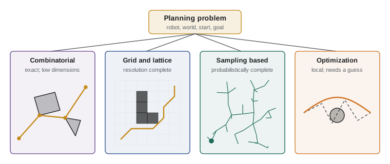
Planners are compared on two theoretical properties. A planner is complete if, whenever a solution exists, it finds one in finite time, and whenever none exists, it reports failure. Complete planners exist for some problems, but in high dimensions they are too slow to use. Weaker guarantees are therefore common. A planner is resolution complete if it is complete at the resolution of its discretization: a grid search finds a path if one exists through the grid cells, but may miss a path through a gap narrower than a cell. A planner is probabilistically complete if the probability of finding an existing solution tends to one as it runs longer, which is the guarantee offered by the sampling-based methods of lessons 6 and 7.
Optimality asks whether the solution found is the best one under the chosen cost. Dijkstra's algorithm and A* with an admissible heuristic are optimal on their graph. RRT is not: it finds a path quickly but the path is usually far from the shortest. RRT* is asymptotically optimal, meaning its solution converges to the optimum as it runs longer. In practice optimality is always relative to the model. A path that is optimal on a coarse grid may be 8 per cent longer than the true shortest path, and a path that is shortest may pass uncomfortably close to obstacles, so practical cost functions usually combine length with clearance, smoothness or time.
Worked problem
Resolution and missed gaps
A robot is modelled as a point after obstacles are inflated by its radius. A doorway leaves a free gap 0.25 m wide. Will a grid planner find the doorway with 0.1 m cells, 0.2 m cells and 0.3 m cells, if a cell is free only when it is entirely in free space?
Show solution
- A gap of width w contains at least one fully free column of cells if the cell size c satisfies roughly \( c \le w/2 \) in the worst alignment, since the cell boundaries may straddle the gap edges.
- With 0.1 m cells: 0.1 ≤ 0.125, so at least one free column exists whatever the alignment; the doorway is found.
- With 0.2 m cells: a free cell exists only if the grid happens to align with the gap; in the worst case both partial cells are marked occupied.
- With 0.3 m cells: no cell fits inside 0.25 m, so the doorway is always blocked.
Answer: Found reliably at 0.1 m, only sometimes at 0.2 m, never at 0.3 m. A resolution-complete planner can only promise paths through gaps comfortably wider than its cells.
Why planning is hard
The general problem is computationally hard. Reif showed in 1979 that the generalized mover's problem, planning for a robot made of many independently moving polyhedral parts, is PSPACE-hard, which means no efficient algorithm is expected to exist. Schwartz and Sharir's 'piano mover's' papers in the early 1980s gave complete algorithms whose running time is polynomial in the number of obstacles but doubly exponential in the number of degrees of freedom, and Canny's roadmap algorithm of 1988 improved this to singly exponential. These results explain the shape of the field. Exact, complete methods are practical only for low-dimensional problems such as a point or polygon robot in the plane. Everything else relies on approximation: discretize the space and search a grid or lattice, sample random configurations and connect them, or optimize a trajectory locally from an initial guess.
The difficulty comes from the size of the configuration space, which grows exponentially with dimension. A grid with 100 cells per axis has \( 10^{4} \) cells in two dimensions, \( 10^{6} \) in three and \( 10^{14} \) in seven. No computer can enumerate a seven-dimensional grid at that resolution, which is why arm planners do not use grids. Collision checking adds a second cost: each candidate configuration must be tested against the world, and for a detailed arm and a cluttered scene that test can take tens of microseconds. A planner that tests a million configurations spends tens of seconds just on collision checks, so good planners are as much about checking few configurations as about clever search.
Worked problem
How big is the grid?
A planner discretizes each joint of an arm into 1° steps over a 360° range. How many cells does the configuration grid have for 2, 3 and 6 joints, and how long would it take merely to visit every cell at \( 10^{8} \) cells per second?
Show solution
- Cells per axis: 360.
- Two joints: \( 360^2 \approx 1.3 \times 10^{5} \), visited in about 1 ms.
- Three joints: \( 360^3 \approx 4.7 \times 10^{7} \), about 0.5 s.
- Six joints: \( 360^6 \approx 2.2 \times 10^{15} \), about \( 2.2 \times 10^{7} \) s, which is roughly eight months.
Answer: Milliseconds for two joints, half a second for three, eight months for six. This is the curse of dimensionality, and it is why sampling-based planners dominate for arms.
The families of methods
Combinatorial methods build an exact representation of free space and search it. Visibility graphs and cell decompositions, met in lesson 2, solve a point or polygon robot in the plane exactly and optimally, but they do not scale. Grid and lattice methods, lessons 3 to 5, discretize the space and search the resulting graph with Dijkstra or A*; they dominate for mobile robots, where the configuration space is two or three dimensional. Sampling-based methods, lessons 6 and 7, avoid building the whole space and instead sample configurations at random, connecting them into a roadmap or tree; they dominate for arms and other high-dimensional systems. Optimization-based methods, lesson 9, start from an initial path and improve it by minimizing a cost subject to constraints; they produce smooth, high-quality motions but may get stuck in local minima.
Real systems combine these. A mobile robot typically runs a global planner on a cost map (lesson 5) and a local planner or controller that reacts to obstacles in real time (lesson 12). An arm typically samples a collision-free path with RRT-Connect and then smooths it by shortcutting and optimization (lessons 7, 9 and 11). Choosing and combining methods for a given robot, environment and timing budget is the real skill, and the capstone in lesson 12 practises it.
# Tiny planning problem: a point robot on a 6 x 6 grid; count free cells and check reachability by flood fill
grid = ["......",
        ".####.",
        ".#....",
        ".#.##.",
        "...#..",
        "####.."]
free = [(r, c) for r in range(6) for c in range(6) if grid[r][c] == "."]
start, goal = (0, 0), (5, 5)
seen = {start}; frontier = [start]
while frontier:
    r, c = frontier.pop()
    for dr, dc in ((1, 0), (-1, 0), (0, 1), (0, -1)):
        n = (r + dr, c + dc)
        if 0 <= n[0] < 6 and 0 <= n[1] < 6 and grid[n[0]][n[1]] == "." and n not in seen:
            seen.add(n); frontier.append(n)
print("free cells:", len(free), "of 36")
print("cells reachable from start:", len(seen))
print("goal reachable:", goal in seen)free cells: 23 of 36 cells reachable from start: 23 goal reachable: True
From problem to deployed planner
A planner in a real robot sits in a loop. Perception updates the world model; the planner produces a path or trajectory; a controller tracks it; and the cycle repeats, often several times a second for mobile robots. This changes what matters. A planner that finds the optimal path in two seconds may be worse than one that finds a good path in 50 milliseconds, because the world will have changed by the time the slow answer arrives. Planners are therefore judged on success rate, planning time (and its worst case, not only its average), path quality, and how gracefully they fail. A planner that reports 'no path' quickly and clearly lets the rest of the system react, for example by asking for a different goal or clearing a blocked aisle; one that searches for ten seconds before timing out does not.
The rest of this course builds the toolkit lesson by lesson: configuration space (lesson 2), graph search (lessons 3 and 4), grids and lattices (lesson 5), sampling (lessons 6 and 7), collision checking (lesson 8), optimization (lesson 9), nonholonomic planning (lesson 10), manipulators and dynamic environments (lesson 11), and finally the design of a complete planning system (lesson 12).
Common mistakes
MistakeTreating a path and a trajectory as the same thing
InsteadA path has no timing; a trajectory adds time, velocity and acceleration. Plan the one the controller needs.
MistakePlanning for the robot's centre point and forgetting its size
InsteadPlan in configuration space, or inflate obstacles by the robot's radius for a disc robot.
MistakeChoosing a grid planner for a seven-joint arm
InsteadGrids explode with dimension; use sampling-based or optimization methods above about four dimensions.
MistakeReporting a planner as complete because it found every test path
InsteadCompleteness is a guarantee about all problems; most practical planners are only resolution or probabilistically complete.
MistakeJudging planners only by average planning time
InsteadWorst-case time and failure behaviour matter more in a robot that must react.
Summary and key terms
- Motion planning finds a collision-free, feasible motion from a start to a goal, given models of the robot and the world.
- A path is a geometric curve of configurations; a trajectory adds timing.
- Constraints include collisions, joint limits, nonholonomic velocity limits, dynamics and task requirements.
- Complete planners guarantee an answer; resolution-complete and probabilistically complete planners give weaker, practical guarantees.
- Optimality is relative to the cost and the discretization; practical costs mix length, clearance, smoothness and time.
- The general problem is PSPACE-hard and the configuration space grows exponentially with dimension.
- Grid, sampling and optimization methods each suit different dimensions and needs, and real systems combine them.
- Motion planning
- Computing a feasible motion from a start to a goal that avoids obstacles.
- Configuration
- A complete specification of the position of every part of the robot.
- Path
- A continuous curve of configurations without timing.
- Trajectory
- A path with timing, giving configuration as a function of time.
- Nonholonomic constraint
- A constraint on velocities that cannot be integrated into a constraint on positions.
- Kinodynamic planning
- Planning that respects both kinematic and dynamic limits.
- Complete
- Guaranteed to find a solution if one exists and to report failure otherwise.
- Resolution complete
- Complete at the resolution of the planner's discretization.
- Probabilistically complete
- Probability of finding an existing solution tends to one with more time.
- Asymptotically optimal
- Solution cost converges to the optimum as planning time grows.
Practice problems
Work each problem on paper first, then reveal the answer to check.
What is the configuration space dimension of a planar robot that must care about its heading?
Show answer
Three: x, y and θ.
Give an example of a nonholonomic constraint.
Show answer
A car cannot move sideways.
What does a trajectory contain that a path does not?
Show answer
Timing, and hence velocities and accelerations.
A grid has 50 cells per axis. How many cells in four dimensions?
Show answer
\( 50^4 = 6.25 \times 10^{6} \).
Which kind of completeness do sampling-based planners offer?
Show answer
Probabilistic completeness.
Why might a grid planner miss a narrow doorway?
Show answer
The gap is narrower than the cells, so no cell is fully free.
Name two costs a practical planner might combine.
Show answer
Path length and clearance, or time and smoothness.
What did Reif show about the generalized mover's problem?
Show answer
It is PSPACE-hard.
What is the dimension of a 6-joint arm on a fixed base?
Show answer
Six.
Why is fast failure reporting useful?
Show answer
It lets the rest of the system react, for example by changing the goal.
Lesson quiz · 5 questions
Score 60% or more to complete this lesson.
Create a free account to save your progress, take quizzes and earn a certificate.