
ROB-340 · Lesson 6 of 12 · 28 min
EKF-SLAM
EKF-SLAM was the first practical SLAM algorithm and, through the 1990s and early 2000s, the standard one. It applies the extended Kalman filter of ROB-310 lesson 6 to a state vector that contains both the robot pose and the positions of all the landmarks. Its great virtue is that it represents the correlations between all of these explicitly, in one covariance matrix, which is exactly what makes SLAM work. Its great weakness is that this matrix grows with the square of the number of landmarks, and that linearization errors accumulate and cannot be undone. Few new systems use plain EKF-SLAM today, but understanding it is the clearest way to see how SLAM behaves: how uncertainty grows while exploring, how it collapses on loop closure, and why the correlations matter. Filter-based visual-inertial odometry, such as the MSCKF, still uses the same machinery.
The state vector
For a planar robot with N point landmarks, the EKF-SLAM state is the robot pose followed by each landmark's position:
so it has \( 3 + 2N \) entries. The belief is a Gaussian with mean \( \boldsymbol{\mu} \) and a \( (3 + 2N) \times (3 + 2N) \) covariance \( \Sigma \). The covariance has a block structure: the robot's own uncertainty in the top-left 3 × 3 block, each landmark's uncertainty in a 2 × 2 block on the diagonal, and the off-diagonal blocks holding the correlations between the robot and each landmark and between every pair of landmarks. Those off-diagonal blocks are the heart of the method.
Worked problem
How big is the EKF-SLAM covariance?
An EKF-SLAM map has 500 landmarks. How many entries does the covariance have, and how much memory in double precision? What about 5,000 landmarks?
Show solution
- State size: \( 3 + 2 \times 500 = 1003 \).
- Covariance entries: \( 1003^2 \approx 1.0 \times 10^6 \); at 8 bytes each, about 8 MB.
- For 5,000 landmarks: state size 10,003, entries about \( 1.0 \times 10^8 \), about 800 MB.
Answer: About 8 MB for 500 landmarks but 800 MB for 5,000. Ten times more landmarks means a hundred times more memory, and each update touches the whole matrix, so computation grows the same way.
Prediction
When the robot moves, only its pose changes; the landmarks are assumed static. The prediction step therefore applies the motion model to the first three entries of the mean and leaves the landmark entries unchanged. The motion Jacobian is the identity everywhere except the top-left 3 × 3 block \( G_x \), so the covariance update
changes only the robot block and the robot-landmark correlation blocks (the first three rows and columns), where F maps the 3 × 3 motion noise R into the full state. A careful implementation updates just those rows and columns, which costs \( O(N) \) rather than \( O(N^2) \). The robot's uncertainty grows with each motion, and through the correlation blocks the filter remembers how that uncertainty relates to the landmarks already seen.
Observing and adding landmarks
A range-bearing sensor measures each landmark's distance r and bearing \( \phi \) relative to the robot. For landmark j at \( (m_x, m_y) \), with \( \delta = (m_x - x, m_y - y) \) and \( q = \delta^{\mathsf{T}}\delta \), the predicted measurement is
Its Jacobian has non-zero entries only in the robot's three columns and the landmark's two columns, which makes it sparse, but the Kalman gain \( K = \Sigma H^{\mathsf{T}} (H \Sigma H^{\mathsf{T}} + Q)^{-1} \) is dense, because \( \Sigma \) is dense. The update \( \Sigma \gets (I - KH)\Sigma \) therefore changes every entry of the covariance: observing one landmark adjusts the estimates of the robot and of every landmark correlated with it. That is how information propagates through the map, and it is also why each update costs \( O(N^2) \).
When a landmark is seen for the first time, it is added to the state. Its initial position comes from inverting the measurement model: \( m_x = x + r\cos(\phi + \theta) \), \( m_y = y + r\sin(\phi + \theta) \). Its covariance and its correlation with everything else come from propagating the robot's covariance and the measurement noise through the Jacobians of this inverse model. A new landmark therefore starts out at least as uncertain as the robot was when it saw it, and it is immediately correlated with the robot pose.
Worked problem
Initializing a landmark
The robot is at (5.0, 2.0) m with heading 30°. It sees a new landmark at range 4.0 m and bearing −30°. Where is the landmark placed?
Show solution
- Absolute bearing: \( \theta + \phi = 30^{\circ} - 30^{\circ} = 0^{\circ} \).
- \( m_x = 5.0 + 4.0\cos 0^{\circ} = 9.0 \) m.
- \( m_y = 2.0 + 4.0\sin 0^{\circ} = 2.0 \) m.
Answer: At (9.0, 2.0) m. Its uncertainty includes the robot's own uncertainty: a 2° heading error alone would place it about \( 4 \times 0.035 = 0.14 \) m to the side.
How uncertainty evolves
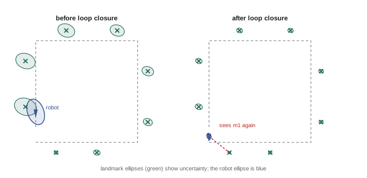
EKF-SLAM shows the characteristic behaviour of all SLAM methods very clearly. While the robot explores new territory, its pose uncertainty grows with odometry, and each new landmark is initialized with an uncertainty at least as large as the robot's at that moment, so landmarks mapped later in an excursion are more uncertain. When the robot returns and re-observes a landmark it mapped early, when it was well localized, its pose uncertainty collapses, and because of the correlations, the uncertainties of all the landmarks seen along the way shrink too. This loop closure effect is the signature of correctly maintained correlations.
import numpy as np
rng = np.random.default_rng(7)
LM = np.array([[x, y] for x in (0, 10, 20) for y in (-3, 13)] + [[-3, 5], [23, 5]], float)
N = len(LM); n = 3 + 2 * N
mu = np.zeros(n); S = np.eye(n) * 1e6; S[:3, :3] = 0            # landmarks unknown, robot known
seen = np.zeros(N, bool); true = np.zeros(3)
Rm = np.diag([0.02, 0.02, np.radians(0.5)]) ** 2; Q = np.diag([0.1, np.radians(1)]) ** 2
def wrap(a): return (a + np.pi) % (2 * np.pi) - np.pi
path = [(1, 0)] * 20 + [(1, np.pi / 2 / 5)] * 5 + [(1, 0)] * 5 + [(1, np.pi / 2 / 5)] * 5 + [(1, 0)] * 20 + [(1, np.pi / 2 / 5)] * 5 + [(1, 0)] * 5 + [(1, np.pi / 2 / 5)] * 5 + [(1, 0)] * 3
report = {}
for k, (v, w) in enumerate(path):
    true += [v * np.cos(true[2]), v * np.sin(true[2]), w]; true[2] = wrap(true[2])
    vm, wm = v + rng.normal(0, 0.02), w + rng.normal(0, np.radians(0.5))
    th = mu[2]
    mu[:3] += [vm * np.cos(th), vm * np.sin(th), wm]; mu[2] = wrap(mu[2])
    G = np.eye(n); G[0, 2] = -vm * np.sin(th); G[1, 2] = vm * np.cos(th)
    S = G @ S @ G.T; S[:3, :3] += Rm
    for j in range(N):
        d = LM[j] - true[:2]; r = np.hypot(*d)
        if r > 6: continue
        z = np.array([r, wrap(np.arctan2(d[1], d[0]) - true[2])]) + rng.normal(0, [0.1, np.radians(1)])
        i = 3 + 2 * j
        if not seen[j]:
            mu[i:i + 2] = mu[:2] + z[0] * np.array([np.cos(z[1] + mu[2]), np.sin(z[1] + mu[2])]); seen[j] = True
        dd = mu[i:i + 2] - mu[:2]; q = dd @ dd; sq = np.sqrt(q)
        zh = np.array([sq, wrap(np.arctan2(dd[1], dd[0]) - mu[2])])
        H = np.zeros((2, n))
        H[:, :3] = np.array([[-dd[0] / sq, -dd[1] / sq, 0], [dd[1] / q, -dd[0] / q, -1]])
        H[:, i:i + 2] = np.array([[dd[0] / sq, dd[1] / sq], [-dd[1] / q, dd[0] / q]])
        K = S @ H.T @ np.linalg.inv(H @ S @ H.T + Q)
        inn = z - zh; inn[1] = wrap(inn[1])
        mu = mu + K @ inn; S = (np.eye(n) - K @ H) @ S
    if k in (55, len(path) - 1):
        report[k] = np.sqrt(np.trace(S[:2, :2]))
print("robot position std before closing the loop: %.2f m" % report[55])
print("robot position std after closing the loop:  %.2f m" % report[len(path) - 1])
print("final position error: %.2f m; landmarks mapped: %d" % (np.hypot(*(mu[:2] - true[:2])), seen.sum()))robot position std before closing the loop: 0.91 m robot position std after closing the loop: 0.14 m final position error: 0.15 m; landmarks mapped: 8
Why EKF-SLAM fails at scale
EKF-SLAM has three well-known limitations. The first is cost: memory and each update are \( O(N^2) \), which limits a single filter to a few hundred landmarks in real time. Submapping methods split the world into local maps of bounded size, each with its own filter, and join them; sparse extended information filters exploit the fact that the information matrix (the inverse covariance) is nearly sparse. The second is linearization: the EKF linearizes at its current estimate and cannot revisit that decision, so errors in heading made early in a loop are frozen into the map. Inconsistency results, meaning the filter's covariance becomes smaller than its actual error, and Huang, Mourikis and Roumeliotis showed in 2008 that standard EKF-SLAM gains spurious information about heading because the linearization points change between updates. The third is data association: a single wrong association is incorporated permanently and, by shrinking the covariance, makes later corrections harder.
These limitations motivated the move to particle filters (lesson 7) and, decisively, to graph-based optimization (lesson 8), which revisits linearization points, scales with sparse solvers and can detect and remove bad constraints. Filters survive where their low latency and constant memory matter most, notably in visual-inertial odometry, where the multi-state constraint Kalman filter (MSCKF, Mourikis and Roumeliotis, 2007) keeps a sliding window of recent camera poses instead of landmarks and remains popular on phones, headsets and drones.
Worked problem
Update cost and real-time limits
An EKF-SLAM update costs roughly \( (3 + 2N)^2 \) floating-point operations times a constant of about 10. A processor sustains \( 10^{9} \) such operations per second for this code. With 20 landmark observations per scan and 10 scans per second, what is the largest map that runs in real time?
Show solution
- Updates per second: \( 20 \times 10 = 200 \).
- Budget per update: \( 10^{9}/200 = 5 \times 10^{6} \) operations.
- Require \( 10(3 + 2N)^2 \le 5 \times 10^{6} \), so \( 3 + 2N \le 707 \), \( N \le 352 \).
Answer: About 350 landmarks. Beyond that, the filter falls behind real time, which is why EKF-SLAM is limited to small maps or split into submaps.
| Property | EKF-SLAM | Consequence |
|---|---|---|
| State | Robot pose plus all landmark positions | Correlations represented explicitly |
| Memory | \( O(N^2) \) | Hundreds of landmarks per filter |
| Update cost | \( O(N^2) \) per observation | Real-time limits on map size |
| Linearization | Once, at the current estimate | Errors frozen in; inconsistency |
| Data association | Committed permanently | One error can corrupt the map |
| Loop closure | Automatic through correlations | Uncertainty collapses everywhere |
Common mistakes
MistakeUpdating the full covariance during prediction
InsteadOnly the robot rows and columns change; update them in O(N).
MistakeInitializing a new landmark with a small fixed covariance
InsteadPropagate the robot covariance and measurement noise so it is correctly correlated.
MistakeForgetting to wrap bearing innovations into ±π
InsteadWrap angles, or the filter makes huge wrong corrections.
MistakeTrusting a shrinking EKF-SLAM covariance as proof of accuracy
InsteadCheck consistency with NEES on simulated runs; EKF-SLAM tends to be overconfident.
MistakeUsing one global EKF for thousands of landmarks
InsteadUse submaps or a graph-based method.
Summary and key terms
- EKF-SLAM estimates a state of the robot pose plus all landmark positions with a single Gaussian.
- Its covariance holds the correlations between robot and landmarks and among landmarks, which make loop closure work.
- Prediction changes only the robot block and its correlations, at O(N) cost.
- A landmark observation updates every entry of the covariance, at O(N²) cost.
- New landmarks are initialized from the inverse measurement model, inheriting the robot's uncertainty.
- Uncertainty grows while exploring and collapses across the map when an early landmark is re-observed.
- Quadratic cost, frozen linearization errors and permanent data association errors limit EKF-SLAM to small maps.
- EKF-SLAM
- SLAM using an extended Kalman filter over the robot pose and landmark positions.
- Augmented state
- A state vector extended to include the map as well as the robot.
- Landmark initialization
- Adding a newly seen landmark to the state from its first measurement.
- Range-bearing measurement
- A measurement of a landmark's distance and direction from the robot.
- Cross-covariance
- An off-diagonal covariance block linking two parts of the state.
- Inconsistency
- A filter whose covariance is smaller than its actual errors.
- Submapping
- Splitting a large map into bounded local maps to limit cost.
- Information matrix
- The inverse of the covariance matrix.
- MSCKF
- A filter that keeps a window of past camera poses for visual-inertial odometry.
- Innovation wrapping
- Bringing angle differences into the range −π to π.
Practice problems
Work each problem on paper first, then reveal the answer to check.
How many entries does the EKF-SLAM state have with 100 landmarks?
Show answer
203.
Approximately how many covariance entries for 100 landmarks?
Show answer
About 41,000.
Which part of the covariance changes in the prediction step?
Show answer
The robot block and the robot-landmark correlations.
Why does one landmark observation change every covariance entry?
Show answer
The Kalman gain is dense because the covariance is dense.
Robot at (0, 0, 90°), landmark at range 3 m, bearing 0°: where is it initialized?
Show answer
At (0, 3) m.
Why are landmarks mapped late in a loop more uncertain?
Show answer
They inherit the robot's larger accumulated uncertainty.
What happens to landmark uncertainties when a loop is closed?
Show answer
They shrink, because of the correlations.
Name one way to scale EKF-SLAM.
Show answer
Submapping or sparse information filters.
What is filter inconsistency?
Show answer
The covariance underestimates the true error.
Name a filter still used for visual-inertial odometry.
Show answer
The MSCKF.
Lesson quiz · 5 questions
Score 60% or more to complete this lesson.
Create a free account to save your progress, take quizzes and earn a certificate.