
ROB-340 · Lesson 3 of 12 · 28 min
Localization in a known map
When a map already exists, the robot's job is to work out where it is in that map and keep track of its pose as it moves. This is the everyday mode of most deployed mobile robots: a warehouse is mapped once during commissioning, and from then on hundreds of robots localize against that map for years. Localization in a known map is much easier than SLAM, because the map is fixed and trusted, but it still has to cope with sensor noise, odometry drift, people and pallets that are not in the map, symmetric corridors that look identical, and the occasional robot that is switched off and carried somewhere else. This lesson turns the Monte Carlo localization of ROB-310 lesson 8 into a practical tool: how it is configured, how it fails, and how scan matching complements it.
Position tracking, global localization and the kidnapped robot
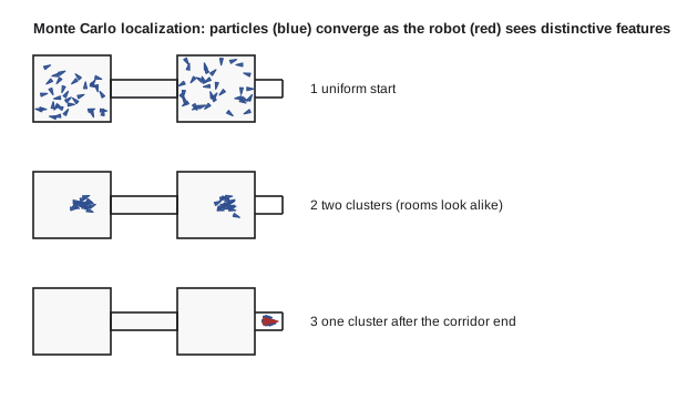
Localization problems come in three levels of difficulty. In position tracking, the initial pose is known approximately and the job is to follow it; a Gaussian filter such as an EKF often suffices, because the belief stays unimodal. In global localization, the robot starts with no idea where it is and must find out from scratch; the belief is initially spread over the whole map and is usually multimodal while the robot is in places that look alike. In the kidnapped robot problem, the robot is confidently localized and then moved without being told (picked up, pushed, or transported in a lift); the filter must first notice that its belief is wrong and then recover. Particle filters handle all three, which is why Monte Carlo localization (MCL), introduced by Dellaert, Fox, Burgard and Thrun in 1999, is the standard method.
Monte Carlo localization in practice
MCL represents the belief with a set of particles, each a candidate pose \( (x, y, \theta) \) with a weight. Each cycle has three steps. First, every particle is moved by the odometry reading with random noise drawn from the motion model, so the cloud spreads to reflect odometry uncertainty. Second, each particle is weighted by how well the current laser scan matches the map from that particle's pose, using a sensor model. Third, particles are resampled in proportion to their weights, so that unlikely poses die out and likely ones multiply. ROB-310 derived each step; here the emphasis is on the choices that make it work on a real robot.
The sensor model is usually the likelihood field (ROB-310 lesson 4): each beam endpoint is projected into the map, and its likelihood is a Gaussian in its distance to the nearest occupied cell, mixed with a uniform term for random returns. The distance to the nearest obstacle is precomputed for every cell, so each beam costs a single lookup. Using every beam of a 1,000-point scan in every particle would be slow and would make the filter overconfident, because neighbouring beams are not independent; implementations therefore use a subset (the ROS AMCL default was 60 beams) and often temper the product of likelihoods.
Adaptive particle counts and recovery
How many particles are needed? Global localization in a large building may need tens of thousands, while tracking a well-localized robot needs only a few hundred. KLD-sampling (Fox, 2003) adapts the count on the fly: during resampling it keeps drawing particles until the number of distinct histogram bins they occupy implies, through the Kullback-Leibler divergence bound, that the sample approximates the true belief to a chosen accuracy. When the particles are spread out, many bins are occupied and many particles are drawn; when they are concentrated, few are needed.
Recovery from kidnapping needs particles where the robot really is, which a converged filter no longer has. Augmented MCL keeps two running averages of the measurement likelihood, a short-term and a long-term one. When the short-term average falls well below the long-term one, the scans have suddenly stopped matching, and the filter injects random particles across the map in proportion to the drop. The ROS AMCL parameters recovery_alpha_slow and recovery_alpha_fast set the two averaging rates; both default to zero, which disables recovery, and setting them to small values such as 0.001 and 0.1 enables it.
Worked problem
How many random particles to inject
An augmented MCL filter has long-term average likelihood \( w_{slow} = 0.020 \) and short-term average \( w_{fast} = 0.006 \) after the robot is pushed. With 2,000 particles, how many are replaced by random ones, using the rule probability \( = \max(0, 1 - w_{fast}/w_{slow}) \)?
Show solution
- Ratio: \( 0.006/0.020 = 0.30 \).
- Injection probability: \( 1 - 0.30 = 0.70 \).
- Expected random particles: \( 0.70 \times 2000 = 1400 \).
Answer: About 1,400 of 2,000 particles are re-drawn uniformly over free space, giving the filter a good chance of finding the true pose in the next few scans. As matching improves, the short-term average recovers and injection stops.
Configuring AMCL
The ROS 2 Nav2 stack ships nav2_amcl, a direct descendant of the original ROS AMCL. Its behaviour is controlled by a few groups of parameters, and most localization problems in practice trace back to one of them.
| Parameter group | Examples | Effect when set badly |
|---|---|---|
| Motion model noise | alpha1 to alpha5, robot_model_type | Too low: overconfident, fails after slip. Too high: particles spread and wander |
| Sensor model | laser_model_type (likelihood_field), max_beams, sigma_hit, z_hit, z_rand | Too few beams or wrong sigma: poor or overconfident weighting |
| Particle count | min_particles, max_particles, pf_err, pf_z | Too few: loses track in large or ambiguous maps |
| Update thresholds | update_min_d, update_min_a | Too large: rare updates; too small: wasted computation and over-correction |
| Recovery | recovery_alpha_slow, recovery_alpha_fast | Zero: cannot recover from kidnapping |
| Resampling | resample_interval | Every update: particle depletion; too rarely: degenerate weights |
A good tuning order is to calibrate odometry first (lesson 1), set the motion noise from measured drift, check the sensor model by watching particle weights on a recorded run, and only then adjust particle counts and thresholds. Recorded data (rosbag2) makes this repeatable: the same run can be replayed with different parameters and the resulting trajectories compared.
# nav2_amcl parameters (excerpt) - a typical starting point for a 2-D lidar robot
amcl:
  ros__parameters:
    robot_model_type: "nav2_amcl::DifferentialMotionModel"
    alpha1: 0.15   # rotation noise from rotation
    alpha2: 0.10   # rotation noise from translation
    alpha3: 0.15   # translation noise from translation
    alpha4: 0.10   # translation noise from rotation
    laser_model_type: "likelihood_field"
    max_beams: 60
    min_particles: 500
    max_particles: 3000
    update_min_d: 0.20      # distance moved (m) before an update
    update_min_a: 0.20      # radians of rotation before an update
    recovery_alpha_slow: 0.001
    recovery_alpha_fast: 0.1
    set_initial_pose: false
Symmetry and ambiguity
Some environments are hard to localize in no matter how good the filter. Long identical corridors, rows of identical racks, and symmetric rooms produce several poses that explain the scans equally well. A particle filter correctly keeps all of them alive until the robot sees something that breaks the symmetry, but if it resamples aggressively with too few particles, it can lock onto the wrong one by chance. Remedies include more particles in ambiguous areas, slower resampling, adding distinctive features (reflectors, fiducial markers or simply a sign on the wall), using a second sensor such as Wi-Fi signal strength or a ceiling camera for coarse position, and giving the robot a known starting pose at its charger.
Worked problem
Detecting an ambiguous belief
After an update, an MCL filter's particles form two clusters: 1,200 particles near (12.0, 4.0) and 800 near (36.0, 4.0), each with a spread of about 0.1 m. What is the mean particle position, and why is reporting it dangerous?
Show solution
- Mean x: \( (1200 \times 12 + 800 \times 36)/2000 = (14400 + 28800)/2000 = 21.6 \) m.
- Mean y: 4.0 m.
- The point (21.6, 4.0) lies between the clusters, 9.6 m from one and 14.4 m from the other, where the robot almost certainly is not.
Answer: The mean, (21.6, 4.0), is a pose no particle supports. A multimodal belief must be summarized by its clusters, and navigation should wait or act to disambiguate rather than plan from the mean.
Scan matching as a localization tool
An alternative or complement to particle filters is scan matching: aligning the current scan directly with the map to find the pose that fits best. Iterative closest point (ICP), introduced for robotics by Besl and McKay and by Chen and Medioni in the early 1990s, repeatedly pairs each scan point with its nearest map point and solves for the rigid transform that minimizes the distances. Correlative scan matching (Olson, 2009) instead evaluates the match score over a grid of candidate poses, which is slower but robust to poor initial guesses and naturally gives a covariance. The normal distributions transform (NDT, Biber and Strasser, 2003) represents the map as a grid of Gaussians, which gives a smooth objective. Lesson 9 covers these methods in depth for lidar SLAM.
Scan matching gives a single best pose rather than a distribution, so it cannot handle global ambiguity on its own, but near the right answer it is more precise than a particle filter with a coarse sensor model. Many production systems therefore use a particle filter or a global search for robustness and a scan matcher for precision, or replace AMCL entirely with a scan-to-map matcher seeded by odometry, as in localization modes of Cartographer and slam_toolbox.
Dynamic environments
Real maps are never perfectly current. People walk past, forklifts park, pallets appear and disappear, and doors open and close. Scans that hit these objects disagree with the map and pull the estimate the wrong way. The likelihood-field model's uniform mixture component and beam-skipping (ignoring beams that most particles agree are unexplained) give some robustness. Better still is to filter out dynamic objects before localization, using detected people and vehicles from perception, or to localize against the parts of the map that change least, such as walls and pillars, rather than shelf contents. Lesson 11 returns to long-term map maintenance.
import numpy as np
rng = np.random.default_rng(3)
# 10 m x 6 m room with a 1 m square pillar at (7, 1.5)-(8, 2.5); robot has 8 range beams
ANG = np.arange(8) * np.pi / 4
def ranges(x, y, th):
    out = []
    for a in ANG:
        dx, dy = np.cos(th + a), np.sin(th + a); t = 0.0
        while t < 12:
            px, py = x + t * dx, y + t * dy
            if not (0 < px < 10 and 0 < py < 6) or (7 < px < 8 and 1.5 < py < 2.5): break
            t += 0.05
        out.append(t)
    return np.array(out)
N = 2000
P = np.column_stack([rng.uniform(0, 10, N), rng.uniform(0, 6, N), rng.uniform(-np.pi, np.pi, N)])
true = np.array([2.0, 3.0, 0.0])
for step in range(12):
    true[0] += 0.4                                       # robot drives +x, 0.4 m per step
    P[:, 0] += 0.4 * np.cos(P[:, 2]) + rng.normal(0, 0.05, N)
    P[:, 1] += 0.4 * np.sin(P[:, 2]) + rng.normal(0, 0.05, N)
    P[:, 2] += rng.normal(0, 0.05, N)
    z = ranges(*true) + rng.normal(0, 0.05, 8)
    w = np.array([np.exp(-np.sum((ranges(*p) - z) ** 2) / (2 * 0.3 ** 2)) for p in P]) + 1e-300
    P = P[rng.choice(N, N, p=w / w.sum())]
    if step in (0, 2, 5, 11):
        err = np.hypot(P[:, 0] - true[0], P[:, 1] - true[1])
print("step %2d: %4.0f%% of particles within 0.3 m of the true position" % (step + 1, 100 * np.mean(err < 0.3)))step 1: 0% of particles within 0.3 m of the true position step 3: 90% of particles within 0.3 m of the true position step 6: 99% of particles within 0.3 m of the true position step 12: 100% of particles within 0.3 m of the true position
Common mistakes
MistakeReporting the mean of a multimodal particle cloud as the robot's pose
InsteadDetect multiple clusters and wait, or act, to disambiguate.
MistakeLeaving AMCL recovery parameters at zero on robots that can be moved by people
InsteadEnable augmented MCL recovery so the filter can detect and recover from kidnapping.
MistakeUsing every beam of a dense scan in the sensor model
InsteadSubsample beams and temper the likelihood to avoid overconfidence.
MistakeTuning particle counts before calibrating odometry
InsteadCalibrate odometry and set motion noise first, then tune the filter.
MistakeLocalizing against shelf contents that change daily
InsteadRely on stable structure such as walls and pillars, and filter dynamic objects.
Summary and key terms
- Localization problems range from position tracking to global localization to recovering a kidnapped robot.
- Monte Carlo localization moves particles with odometry, weights them with a sensor model and resamples.
- The likelihood-field model scores beam endpoints by their distance to the nearest map obstacle, with a precomputed lookup.
- KLD-sampling adapts the particle count; augmented MCL injects random particles when likelihoods suddenly drop.
- In Nav2, AMCL behaviour is governed by motion noise, sensor model, particle count, update thresholds and recovery parameters.
- Symmetric environments produce multimodal beliefs that must not be summarized by their mean.
- Scan matching (ICP, correlative, NDT) gives precise single poses and complements particle filters.
- Position tracking
- Following a robot's pose from an approximately known start.
- Global localization
- Determining the pose with no prior knowledge of where the robot is.
- Kidnapped robot problem
- Recovering when a localized robot is moved without the filter being told.
- Monte Carlo localization
- Particle-filter localization against a known map.
- AMCL
- Adaptive Monte Carlo localization, the standard ROS implementation.
- Likelihood field
- A sensor model scoring beam endpoints by distance to the nearest obstacle.
- KLD-sampling
- Adapting the number of particles to the spread of the belief.
- Augmented MCL
- MCL that injects random particles when measurement likelihoods drop.
- Scan matching
- Aligning a scan with a map or another scan to estimate pose.
- Multimodal belief
- A belief with several separate likely poses.
Practice problems
Work each problem on paper first, then reveal the answer to check.
Which localization problem starts with no idea of the pose?
Show answer
Global localization.
What are the three steps of each MCL cycle?
Show answer
Move particles with odometry, weight them with the sensor model, resample.
Why does the likelihood-field model precompute distances?
Show answer
So each beam costs one lookup.
What does KLD-sampling adapt?
Show answer
The number of particles.
w_slow = 0.05, w_fast = 0.04: what fraction of particles are injected?
Show answer
20 %.
Which AMCL parameters enable kidnapping recovery?
Show answer
recovery_alpha_slow and recovery_alpha_fast.
Two equal clusters at x = 10 m and x = 30 m: what is the mean x, and is it useful?
Show answer
20 m; no, it lies between the clusters.
Name two scan matching methods.
Show answer
ICP, correlative scan matching or NDT.
Name one way to break symmetry in a corridor.
Show answer
Add a reflector, marker or sign, or use another sensor.
Why should odometry be calibrated before tuning AMCL?
Show answer
Motion noise settings depend on how much odometry really drifts.
Lesson quiz · 5 questions
Score 60% or more to complete this lesson.
Create a free account to save your progress, take quizzes and earn a certificate.