
ROB-340 · Lesson 1 of 12 · 32 min
Mobile robot platforms and odometry
A mobile robot has to answer three questions over and over: where am I, what does the world around me look like, and how do I get where I am going? This course is about the first two. Localization estimates the robot's pose in a map it already has. Mapping builds that map from sensor data. Simultaneous localization and mapping, or SLAM, does both at once, and it is the technology that lets a warehouse robot, a floor-cleaning robot, a planetary rover or a self-driving car operate in places nobody surveyed for it. ROB-310 developed the estimation tools (Bayes filters, Kalman filters, particle filters and factor graphs); this course applies them to the specific problems of mobile robots. Path planning, the third question, belongs to ROB-350.
Everything starts with odometry: the robot's own estimate of how far it has moved since the last instant. Odometry is fast, always available and smooth, and it is also always wrong by a little, with errors that accumulate without bound. Understanding exactly how odometry drifts, and how to calibrate it, is the foundation for every localization and mapping method that follows, because they all use odometry as the motion model that predicts the robot's next pose.
Mobile robot platforms
Most indoor mobile robots use a differential drive: two independently driven wheels on a common axle, with one or more passive casters for balance. It is mechanically simple, can turn on the spot, and its kinematics are easy to model, which is why it dominates warehouse robots, hospital delivery robots and research platforms. Car-like robots use Ackermann steering, which cannot turn in place and has a minimum turning radius, a constraint that matters for planning. Skid-steer robots (tracked or four-wheel vehicles that turn by driving the sides at different speeds) are rugged and common outdoors, but their wheels must slip sideways to turn, which makes their odometry much worse. Omnidirectional platforms with mecanum or omni wheels can move sideways, at the cost of more slip and sensitivity to floor dirt. Legged robots replace wheel odometry with leg odometry from joint encoders and foot contacts, fused with an inertial measurement unit (IMU).
ROB-210 derived the kinematics of these platforms. Here we only need the differential-drive model. With wheel radius r, track width b (the distance between the wheel contact points) and wheel angular speeds \( \omega_L \) and \( \omega_R \), the forward speed and turn rate are
Odometry integrates these speeds over time. In practice the robot reads its wheel encoders at a fixed rate, converts the tick counts since the last reading into distances travelled by each wheel, \( \Delta s_L \) and \( \Delta s_R \), and updates the pose \( (x, y, \theta) \) with
Using the heading at the middle of the step, \( \theta + \Delta\theta/2 \), is a second-order (midpoint) integration that is noticeably more accurate than using the old heading when the robot turns between readings.
Worked problem
Encoder ticks to a pose update
A differential-drive robot has 0.075 m wheel radius, 0.40 m track width and encoders giving 4,096 ticks per wheel revolution (after the gearbox). In one 100 ms update the left wheel advances 1,210 ticks and the right 1,290 ticks. The robot starts at (0, 0, 0). Find its new pose.
Show solution
- Distance per tick: \( 2\pi \times 0.075/4096 = 1.150 \times 10^{-4} \) m.
- \( \Delta s_L = 1210 \times 1.150 \times 10^{-4} = 0.1392 \) m; \( \Delta s_R = 1290 \times 1.150 \times 10^{-4} = 0.1484 \) m.
- \( \Delta s = 0.1438 \) m and \( \Delta\theta = (0.1484 - 0.1392)/0.40 = 0.0230 \) rad.
- Midpoint heading 0.0115 rad: \( x = 0.1438\cos(0.0115) = 0.1438 \) m, \( y = 0.1438\sin(0.0115) = 0.0017 \) m.
Answer: The pose becomes about (0.144 m, 0.002 m, 0.023 rad), a forward speed of about 1.44 m/s and a gentle left turn. Real systems repeat this update 10 to 100 times a second.
Why odometry drifts
Odometry errors come in two kinds. Systematic errors are biases that repeat the same way every time: unequal wheel diameters (from manufacturing tolerance, uneven wear or a heavier load on one side), an actual track width different from the nominal value, misalignment of the wheels, and the finite encoder resolution and sampling rate. Non-systematic errors are random: wheel slip on smooth or wet floors, bumps and cracks, rolling over cables, sideways slip when turning, and the casters pushing the robot off line. Systematic errors dominate on smooth indoor floors and can be calibrated away; non-systematic errors dominate on rough terrain and can only be modelled as noise.
The key property of dead reckoning is that heading errors are the most damaging. A small error in \( \Delta\theta \) at each step accumulates into a heading error that grows with distance, and then every subsequent metre of travel is in a slightly wrong direction, so the position error grows faster than linearly. A heading error \( \delta\theta \) after travelling a distance D gives a lateral position error of about \( D\,\delta\theta \). This is why a cheap gyroscope, which measures heading change directly, so often improves wheel odometry dramatically.
Worked problem
How far off does a small heading error take you?
A robot's odometry has drifted 1.5° in heading by the time it starts a 40 m straight run down an aisle. Assuming no further error, how far off line is it at the end of the aisle?
Show solution
- Convert: \( 1.5^{\circ} = 0.0262 \) rad.
- Lateral error \( \approx D\,\delta\theta = 40 \times 0.0262 = 1.05 \) m.
Answer: About 1 m sideways, more than enough to put the robot into a rack. A heading error of only a degree or two, invisible to the eye, must be corrected by localization within tens of metres.
Track width error causes heading error directly: if the true track width is \( b(1+\epsilon) \) but the software uses b, every computed turn is too large by the fraction \( \epsilon \). Unequal wheel diameters cause the robot to curve gently when it thinks it is driving straight. Both effects are small (a fraction of a percent) but they accumulate on every trip.
import numpy as np
rng = np.random.default_rng(1)

r, b = 0.075, 0.40              # nominal wheel radius and track width (m)
rR_true = r * 1.004             # right wheel 0.4 % larger than nominal
b_true = b * 1.01               # true track 1 % wider than nominal
dt, v, n = 0.02, 1.0, 3000      # 60 s at 1 m/s straight ahead command

x = y = th = 0.0                # odometry estimate
X = Y = TH = 0.0                # true pose
for k in range(n):
    w = v / r                    # commanded wheel speed for straight driving
    wL = wR = w + rng.normal(0, 0.05)   # small common speed noise
    sL, sR = r * wL * dt, r * wR * dt              # what odometry believes
    SL, SR = r * wL * dt, rR_true * wR * dt        # what really happens
    ds, dth = (sR + sL) / 2, (sR - sL) / b
    x += ds * np.cos(th + dth / 2); y += ds * np.sin(th + dth / 2); th += dth
    DS, DTH = (SR + SL) / 2, (SR - SL) / b_true
    X += DS * np.cos(TH + DTH / 2); Y += DS * np.sin(TH + DTH / 2); TH += DTH
print("odometry thinks: x=%.2f m y=%.2f m heading=%.2f deg" % (x, y, np.degrees(th)))
print("truth:           x=%.2f m y=%.2f m heading=%.2f deg" % (X, Y, np.degrees(TH)))
print("position error after %.0f m: %.2f m" % (x, np.hypot(x - X, y - Y)))odometry thinks: x=60.00 m y=0.00 m heading=0.00 deg truth: x=56.65 m y=17.34 m heading=34.04 deg position error after 60 m: 17.66 m
The result is striking: a mismatch of only 0.4 % between the wheels, smaller than normal tire wear, curves the true path by about 34° over 60 m and leaves the robot more than 17 m from where its odometry says it is. The odometry itself shows nothing wrong, which is why such errors must be found by calibration against an external reference.
Calibrating odometry: the UMBmark test
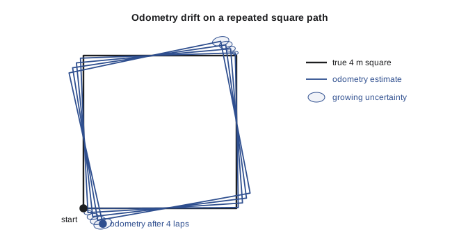
Because systematic errors repeat, they can be measured and removed. The best-known procedure is UMBmark (University of Michigan Benchmark), published by Johann Borenstein and Liqiang Feng in 1996. The robot drives a square path, typically 4 m on a side, several times clockwise and several times counter-clockwise, and its true final position is measured against the start. Unequal wheel diameters and track width error affect the two directions differently: a track width error makes the robot over- or under-turn at each corner in the same sense regardless of direction, so its effect reverses relative to the path, while a diameter mismatch curves every straight leg the same way. Comparing the clockwise and counter-clockwise error clusters separates the two, and simple formulas give correction factors for the wheel diameter ratio and the effective track width.
In practice many teams use a simpler two-step version. First, drive straight a long measured distance (say 10 m) and adjust the average wheel radius until odometry reports the true distance; also note any sideways curve and adjust the right-to-left diameter ratio. Second, spin the robot on the spot through ten full turns and adjust the effective track width until odometry reports exactly 3,600°. The effective track width is usually a little larger than the measured axle length, because the wheel contact patch is not a point and the tires scrub.
Worked problem
Calibrating track width by spinning
A robot with nominal track width 0.400 m is commanded to spin on the spot until odometry reports 10 full turns (3,600°). Measured with a laser on the floor, it actually turned 3,564°. What effective track width should the software use?
Show solution
- Odometry computes \( \Delta\theta = (\Delta s_R - \Delta s_L)/b \), so the reported angle is inversely proportional to the b used.
- The reported angle scales as \( b_{true}/b_{used} \) times the true angle, so \( 3600 = 3564 \times b_{eff}/0.400 \), giving \( b_{eff} = 0.400 \times 3600/3564 \).
- \( b_{eff} = 0.400 \times 1.0101 = 0.4040 \) m.
Answer: Use 0.404 m. With the larger value, the same wheel travel produces a smaller computed turn, so odometry will report the true 3,564° as 3,564°. A 1 % track width correction like this removes most of the heading drift on smooth floors.
Other sources of odometry
Wheel odometry is not the only option, and modern robots usually combine several. Visual odometry (ROB-330 lesson 7) estimates motion from camera images and does not care about wheel slip, but it fails in the dark, on blank walls and during fast motion, and a single camera cannot observe scale. Lidar odometry estimates motion by matching successive laser scans (lesson 9 of this course); it is accurate in structured buildings but can degenerate in long featureless corridors, where every scan looks the same along the corridor axis. Inertial odometry integrates accelerometer and gyroscope readings; gyroscopes are excellent for short-term heading, but double-integrating acceleration drifts quadratically with time, so an IMU alone cannot give position for more than a few seconds. Optical floor sensors (like the sensor in a computer mouse) and ground-penetrating radar are used in some niche applications.
Fusing these sources is exactly the sensor fusion problem of ROB-310 lesson 9. A typical ROS 2 configuration runs the robot_localization package's EKF on the wheel odometry and the IMU yaw rate, producing a smooth, continuous odometry estimate in the odom frame, while a separate localization or SLAM node corrects the accumulated drift by publishing the transform from map to odom. Keeping these two frames separate (following ROS REP 105) means the robot's controller always sees a smooth pose, while the global pose can jump when a correction arrives.
| Odometry source | Strengths | Weaknesses | Typical drift |
|---|---|---|---|
| Wheel encoders | Cheap, always available, high rate | Slip, bumps, calibration errors | 1–5 % of distance indoors |
| Wheel + gyroscope | Much better heading | Gyro bias drift over minutes | 0.5–2 % of distance |
| Visual odometry | Immune to wheel slip | Dark, blank or fast scenes; scale (mono) | About 1 % of distance |
| Lidar odometry | Accurate in structured spaces | Long corridors, open fields | 0.2–1 % of distance |
| IMU alone | Very high rate, no external dependence | Position drifts quadratically | Useful only for seconds |
Modelling odometry uncertainty
Localization and mapping algorithms need odometry with a covariance, not just a value. ROB-310 lesson 3 developed the odometry motion model: the motion between two readings is decomposed into an initial rotation, a translation and a final rotation, each corrupted by noise whose variance grows with the size of the motion. The four noise parameters (often called alpha1 to alpha4 in ROS packages) express how much rotation noise comes from rotation, how much from translation, and so on. Because uncertainty is added at each step, the covariance of the pose grows over time; with heading uncertainty, the uncertainty cloud stretches into the famous banana shape, curved because heading errors push the position sideways. Setting these parameters realistically matters: if they are too small, a filter becomes overconfident and refuses to accept corrections; if they are too large, the robot's particles spread so fast that localization becomes fragile.
Odometry as the motion model for everything that follows
Every method in this course uses odometry in the same role. In Monte Carlo localization (lesson 3), odometry moves the particles, and the sensor model then weighs them against the map. In occupancy grid mapping (lesson 4), the pose estimate tells the mapper where each laser beam started. In EKF-SLAM and particle-filter SLAM (lessons 6 and 7), odometry drives the prediction step. In graph-based SLAM (lesson 8), each odometry measurement becomes an edge constraint between two consecutive poses. The better the odometry, the less work the corrections have to do, the smaller the loops that can be closed reliably, and the longer the robot can survive in places where its sensors see nothing useful. Calibrated, well-modelled odometry is never wasted effort.
Common mistakes
MistakeUsing the nominal axle length as the track width without calibration
InsteadCalibrate the effective track width by spinning the robot through many turns.
MistakeUpdating the pose with the old heading during turns
InsteadUse the midpoint heading, or an exact arc update, for each step.
MistakeTrusting odometry heading for long runs
InsteadFuse a gyroscope and correct drift with localization against a map.
MistakeSetting odometry noise parameters to tiny values
InsteadChoose realistic noise so the filter remains willing to accept corrections.
MistakeAssuming a skid-steer robot's odometry is as good as a differential drive's
InsteadExpect much larger turning errors from sideways slip and model them.
Summary and key terms
- Localization, mapping and SLAM answer where the robot is and what the world looks like; planning (ROB-350) decides how to move.
- Differential-drive odometry converts encoder ticks into wheel distances, then a pose update using the midpoint heading.
- Systematic odometry errors (wheel diameter, track width) repeat and can be calibrated; non-systematic errors (slip, bumps) are random.
- Heading errors are the most damaging because a heading error makes every later metre go the wrong way.
- UMBmark and simple straight-line and spin tests measure wheel-radius and track-width corrections.
- Visual, lidar and inertial odometry complement wheel odometry and are usually fused, publishing a smooth odom frame.
- Odometry uncertainty grows without bound and serves as the motion model for localization and SLAM.
- Odometry
- An estimate of a robot's motion from its own sensors, integrated over time.
- Dead reckoning
- Estimating position by integrating speed and heading from a known start.
- Differential drive
- A platform with two independently driven wheels on a common axle.
- Track width
- The distance between the contact points of a robot's drive wheels.
- Systematic error
- A repeatable bias, such as an incorrect wheel radius, that can be calibrated.
- Non-systematic error
- A random error, such as wheel slip, that must be modelled as noise.
- UMBmark
- A square-path benchmark that separates and calibrates systematic odometry errors.
- Skid steer
- Steering by driving the two sides at different speeds, causing sideways wheel slip.
- odom frame
- The ROS frame in which odometry is continuous but drifts over time.
- Banana distribution
- The curved uncertainty cloud produced by heading uncertainty during motion.
Practice problems
Work each problem on paper first, then reveal the answer to check.
A wheel of radius 0.1 m with 2,000 ticks per revolution: what distance is one tick?
Show answer
About 0.314 mm.
Left wheel 0.50 m, right wheel 0.54 m, track 0.4 m: what is the heading change?
Show answer
0.1 rad.
Why use the midpoint heading in the pose update?
Show answer
It is a more accurate (second-order) integration when the robot turns during the step.
A 2° heading error over a 25 m run gives about what lateral error?
Show answer
About 0.87 m.
Name two systematic odometry errors.
Show answer
Unequal wheel diameters and an incorrect track width.
Name two non-systematic odometry errors.
Show answer
Wheel slip and bumps or cables on the floor.
A spin test reports 3,600° but the robot turned 3,636°. Should the track width used go up or down?
Show answer
Down, to about 0.99 times its value.
Why can't an IMU alone provide position for long?
Show answer
Double-integrating acceleration makes position error grow quadratically with time.
Which ROS frame is continuous but drifts?
Show answer
The odom frame.
What happens if odometry noise parameters are set too small?
Show answer
The filter becomes overconfident and rejects corrections.
Lesson quiz · 5 questions
Score 60% or more to complete this lesson.
Create a free account to save your progress, take quizzes and earn a certificate.