The Kalman filter

The Kalman filter is the Bayes filter for linear systems with Gaussian noise, and in that setting it is exact: no approximation, just a handful of matrix equations that update a mean and a covariance. Published by Rudolf Kálmán in 1960 and soon used to navigate the Apollo spacecraft, it remains the most widely used estimator in engineering. Every phone, drone, car and industrial robot runs some form of it. Even where systems are nonlinear, the extended and unscented filters of lessons 6 and 7 keep the Kalman structure and only change how the means and covariances are propagated. This lesson builds the filter from the one-dimensional case, where the equations reduce to intuitive averaging, up to the full matrix form, and then covers the practical questions every implementer faces: how to choose the noise covariances and how to tell whether the filter is working.

Fusing two Gaussians

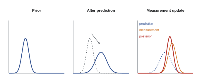
Suppose a robot believes its position is \( \mathcal{N}(\mu_1, \sigma_1^2) \) and then receives a measurement that, on its own, suggests \( \mathcal{N}(\mu_2, \sigma_2^2) \). Multiplying the two Gaussians, as Bayes' rule requires, gives another Gaussian with

The new mean is a weighted average that trusts the more certain source more, and the new variance is smaller than either: inverse variances, called information, simply add. Rewriting the mean as \( \mu = \mu_1 + K(\mu_2 - \mu_1) \) with \( K = \sigma_1^2/(\sigma_1^2 + \sigma_2^2) \) gives the Kalman form: start from the prior, and move toward the measurement by a fraction K of the disagreement. K, the Kalman gain, is near 1 when the prior is vague relative to the measurement and near 0 when the measurement is the noisy one.

The linear Gaussian system model

The Kalman filter assumes the state evolves and is observed linearly, with additive Gaussian noise:

A is the state transition matrix, B maps controls into the state, H is the measurement matrix and Q and R are the process and measurement noise covariances. (Some texts, including Probabilistic Robotics, swap the letters and call process noise R and measurement noise Q; always check a source's convention.) The process noise w represents everything the motion model leaves out, from unmodelled accelerations to wheel slip, and the measurement noise v represents sensor error. Under these assumptions, with a Gaussian initial belief, the belief stays Gaussian forever, and the filter only needs to track its mean \( \boldsymbol{\mu} \) and covariance \( \boldsymbol{\Sigma} \).

The filter equations

The prediction step applies the rules of lesson 1 for linear maps of Gaussians:

The correction step computes the innovation \( \mathbf{y}_t = \mathbf{z}_t - \mathbf{H}\bar{\boldsymbol{\mu}}_t \), the difference between what was measured and what was expected; its covariance \( \mathbf{S}_t = \mathbf{H}\bar{\boldsymbol{\Sigma}}_t\mathbf{H}^{\mathsf{T}} + \mathbf{R} \); the Kalman gain; and the updated belief:

These are the matrix versions of the one-dimensional fusion formulas. The gain matrix K does more than weight: it spreads the correction across all state components according to their covariance with what was measured. A position-only measurement in a filter whose state includes velocity also corrects the velocity, because predicted position and velocity are correlated through the motion model. This is how a Kalman filter estimates quantities it never measures directly. Numerically, the simple covariance update can lose symmetry or positive definiteness through rounding, so careful implementations use the Joseph form \( \boldsymbol{\Sigma}_t = (\mathbf{I} - \mathbf{K}\mathbf{H})\bar{\boldsymbol{\Sigma}}(\mathbf{I} - \mathbf{K}\mathbf{H})^{\mathsf{T}} + \mathbf{K}\mathbf{R}\mathbf{K}^{\mathsf{T}} \), which stays symmetric and positive definite for any gain.

A constant-velocity tracking filter

A common first filter tracks an object moving along a line, such as a robot on a rail or a conveyor item, with state \( \mathbf{x} = [p, v]^{\mathsf{T}} \) of position and velocity, from noisy position measurements every Δt seconds. Assuming velocity is roughly constant but disturbed by random accelerations of spectral density q,

This continuous white-noise acceleration model gives a Q whose structure, with correlated position and velocity noise, follows from integrating random acceleration over a step. The single tuning parameter q expresses how much the velocity is expected to wander: small q gives smooth but sluggish estimates that lag behind real speed changes; large q gives responsive but noisy estimates.

import numpy as np
rng = np.random.default_rng(5)
dt, q, sz, T = 0.1, 0.5, 0.2, 300
A = np.array([[1, dt], [0, 1]]); H = np.array([[1.0, 0.0]])
Q = q*np.array([[dt**3/3, dt**2/2], [dt**2/2, dt]]); R = np.array([[sz**2]])
x = np.array([0.0, 1.0]); mu = np.array([0.0, 0.0]); S = np.diag([1.0, 1.0])
err, nees = [], []
for t in range(T):
    x = A @ x + rng.multivariate_normal([0, 0], Q)           # true motion
    z = H @ x + rng.normal(0, sz, 1)                          # noisy position
    mu = A @ mu; S = A @ S @ A.T + Q                          # predict
    y = z - H @ mu; Sy = H @ S @ H.T + R; K = S @ H.T @ np.linalg.inv(Sy)
    mu = mu + K @ y; IKH = np.eye(2) - K @ H
    S = IKH @ S @ IKH.T + K @ R @ K.T                         # Joseph form
    e = x - mu; err.append(e); nees.append(e @ np.linalg.inv(S) @ e)
err = np.array(err[50:]); nees = np.array(nees[50:])
print("position RMSE: %.3f m (measurement noise %.2f m)" % (np.sqrt(np.mean(err[:, 0]**2)), sz))
print("velocity RMSE: %.3f m/s" % np.sqrt(np.mean(err[:, 1]**2)))
print("steady-state gain:", np.round(K.ravel(), 3))
print("mean NEES: %.2f (expected 2 for a consistent 2-state filter)" % nees.mean())

position RMSE: 0.130 m (measurement noise 0.20 m)
velocity RMSE: 0.410 m/s
steady-state gain: [0.377 0.883]
mean NEES: 2.06 (expected 2 for a consistent 2-state filter)

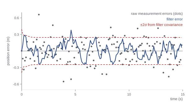
The filter cuts the position error from the raw 0.20 m measurement noise to 0.13 m by averaging over time, and it estimates velocity, which was never measured, to about 0.4 m/s even though the true velocity wanders randomly; a smaller q would smooth the velocity estimate further at the cost of lag when the object really changes speed. The gain settles to a constant: for time-invariant systems the covariance converges, and many embedded implementations simply precompute this steady-state gain, giving a fixed-gain filter (closely related to the classic alpha–beta tracker) that costs only a few multiplications per step.

Tuning Q and R

The measurement noise R can usually be estimated directly by logging a sensor while the true value is constant and computing the variance, then inflating it a little for effects the bench test missed. The process noise Q is harder, because it stands for everything the model does not capture. It is normally tuned: start from a physically motivated value (for example, the typical random acceleration the platform experiences) and adjust until the filter's behaviour is right. The ratio of Q to R is what matters for the estimate; their absolute scale matters for the reported covariance. Too little Q makes the filter overconfident in its model, slow to follow real changes and prone to divergence, where the estimate drifts away while its covariance claims it is accurate. Too much Q makes the estimate jittery, following measurement noise.

Two consistency statistics turn tuning from guesswork into measurement. The normalized innovation squared, \( \text{NIS}_t = \mathbf{y}_t^{\mathsf{T}}\mathbf{S}_t^{-1}\mathbf{y}_t \), can be computed on real data and should average the measurement dimension (1 for a scalar measurement) if the filter is consistent. The normalized estimation error squared, \( \text{NEES}_t = \mathbf{e}_t^{\mathsf{T}}\boldsymbol{\Sigma}_t^{-1}\mathbf{e}_t \), needs the true state and so is used in simulation; it should average the state dimension. An average well above the expected value means the filter is overconfident (Σ too small, usually Q too small); well below means underconfident. In the simulation above the mean NEES is close to 2, the state dimension, as it should be when the filter's models match the simulated world.