
ROB-310 · Lesson 11 of 12 · 31 min
Estimation for manipulation and perception: pose, tracking and data association
Localization asks where the robot is. Many robotic tasks also need to know where other things are: the pose of a part on a conveyor so an arm can pick it, the position and velocity of people near a mobile robot, the location of a tool in the gripper. The same probabilistic tools apply, but two problems become central. The first is estimating an object's full position and orientation from sensor data, often by aligning a model with measured points. The second is data association: when the sensor reports several detections and there are several objects, which detection belongs to which object, and which detections are clutter? This lesson covers point-set alignment and its uncertainty, multi-target tracking with Kalman filters, the main data association methods, and how these ideas appear in manipulation.
Estimating a pose by aligning points
Suppose a robot knows a set of model points on an object, \( \mathbf{p}_i \) in the object frame, such as the corners of a box or the centres of fiducial markers, and its sensor measures the corresponding points \( \mathbf{q}_i \) in the camera frame. The object's pose is the rotation R and translation t that best map model points onto measured points, minimizing
When correspondences are known, this problem has a closed-form solution, often called the Kabsch or Umeyama method. Subtract the centroids \( \bar{\mathbf{p}} \) and \( \bar{\mathbf{q}} \) from each set, form the cross-covariance matrix \( \mathbf{W} = \sum_i (\mathbf{q}_i - \bar{\mathbf{q}})(\mathbf{p}_i - \bar{\mathbf{p}})^{\mathsf{T}} \), take its singular value decomposition \( \mathbf{W} = \mathbf{U}\mathbf{D}\mathbf{V}^{\mathsf{T}} \), and set
The determinant term prevents the solution from being a reflection rather than a rotation. When correspondences are unknown, as with raw lidar or depth-camera points, the iterative closest point (ICP) algorithm alternates two steps: match each measured point to its nearest model point under the current pose estimate, then solve the alignment above for those matches, repeating until the pose stops changing. ICP converges quickly from a good initial guess but can lock onto a wrong alignment from a poor one, so it is usually initialized from a coarser method, such as feature matching or a previous estimate. For camera images, where only 2-D projections of known 3-D points are measured, the corresponding problem is perspective-n-point (PnP), solved by algorithms such as EPnP followed by nonlinear refinement; fiducial markers like AprilTags use exactly this to give a full 6-D pose from a single image.
Worked problem
Translation from centroids
Model points (0, 0), (2, 0) and (0, 1) are measured, with no rotation, at (3, 1), (5, 1) and (3, 2). Find the translation.
Show solution
- Model centroid: \( (2/3, 1/3) \).
- Measured centroid: \( (11/3, 4/3) \).
- With R = I, \( \mathbf{t} = (11/3 - 2/3,\ 4/3 - 1/3) = (3, 1) \).
Answer: The object is translated by (3, 1). With rotation present, the SVD step finds R first, and the translation is then the measured centroid minus the rotated model centroid.
import numpy as np
rng = np.random.default_rng(8)
P = np.array([[0, 0], [0.30, 0], [0.30, 0.20], [0, 0.20], [0.15, 0.25]])   # model points (m)
th = np.radians(25); R_true = np.array([[np.cos(th), -np.sin(th)], [np.sin(th), np.cos(th)]])
t_true = np.array([0.8, 0.4])
def kabsch(P, Q):
    pc, qc = P.mean(0), Q.mean(0)
    U, D, Vt = np.linalg.svd((Q - qc).T @ (P - pc))
    R = U @ np.diag([1, np.linalg.det(U @ Vt)]) @ Vt
    return R, qc - R @ pc
ang, pos = [], []
for trial in range(2000):
    Q = P @ R_true.T + t_true + rng.normal(0, 0.005, P.shape)     # 5 mm measurement noise
    R, t = kabsch(P, Q)
    ang.append(np.degrees(np.arctan2(R[1, 0], R[0, 0])) - 25); pos.append(t - t_true)
ang, pos = np.array(ang), np.array(pos)
print(f"angle error: mean {ang.mean():+.3f} deg, std {ang.std():.3f} deg")
print(f"translation error std (mm): {np.round(pos.std(0)*1000, 2)}")
P4 = P*0.25                                                      # same shape, one quarter the size
a4 = [np.degrees(np.arctan2(*kabsch(P4, P4 @ R_true.T + t_true + rng.normal(0, 0.005, P.shape))[0][[1, 0], 0])) - 25 for _ in range(2000)]
print(f"angle error std for a 4x smaller object: {np.std(a4):.3f} deg")angle error: mean +0.026 deg, std 0.755 deg translation error std (mm): [3.24 2.43] angle error std for a 4x smaller object: 2.949 deg
The Monte Carlo run shows that the estimate is essentially unbiased (a mean angle error of 0.03°) and that 5 mm of point noise gives about 0.76° of angular uncertainty and 2 to 3 mm of translation uncertainty for a 30 cm object, but about 2.9°, almost four times more, for an object a quarter of the size. Angular accuracy scales inversely with the spread of the points, the same geometry that makes a long baseline better for triangulation. This is why grippers pick small parts more reliably with a close-up camera, and why fiducial markers for accurate pose estimation are made as large as practical.
Uncertainty of pose estimates
A pose estimate is only useful for manipulation if its uncertainty is known: an arm inserting a peg into a hole with 0.5 mm clearance needs to know whether the estimated hole position is good to 0.1 mm or 2 mm. Pose covariance can be estimated from the Jacobian of the alignment residuals, \( \boldsymbol{\Sigma} \approx \sigma^2(\mathbf{J}^{\mathsf{T}}\mathbf{J})^{-1} \), the same expression as the information matrix of lesson 10, or by Monte Carlo as above. Rotations need care: covariance is usually expressed in a small three-element rotation error about the estimate rather than in Euler angles or quaternion components. Once a pose and its covariance are available, a Kalman filter can track an object over time, fusing estimates from successive images and propagating with a motion model, constant for a part on a table or constant-velocity for a part on a conveyor.
Tracking multiple targets
A mobile robot moving among people, or a sorting robot watching items on a conveyor, must track many objects at once. A common architecture runs one Kalman filter per track, usually with a constant-velocity model like that of lesson 5, and at each sensor frame performs three tasks: predict every track to the frame time, associate detections with tracks, and update each track with its associated detection. Detections that match no track may start tentative new tracks, and tracks that go unmatched for too long are deleted. A typical confirmation rule is M-of-N: a tentative track is confirmed when it has been matched in at least M of its first N frames, such as 3 of 5, which suppresses tracks started by isolated false detections.
Worked problem
M-of-N confirmation
A detector produces a false detection in a given location with probability 0.1 per frame, independently. With a 2-of-3 confirmation rule, what is the probability that a false detection becomes a confirmed track (assuming the first frame already contains it)?
Show solution
- Confirmation needs at least one more detection in the next two frames.
- Probability of no further detection: \( 0.9^2 = 0.81 \).
- Probability of confirmation: \( 1 - 0.81 = 0.19 \).
- With 3-of-5: needs at least 2 more in the next 4 frames: \( 1 - 0.9^4 - 4(0.1)(0.9^3) = 1 - 0.6561 - 0.2916 = 0.052 \).
Answer: 2-of-3 confirms about 19 % of false starts; 3-of-5 confirms about 5 %, at the cost of confirming real targets two frames later. The rule trades false tracks against latency.
Data association
Data association decides which detection, if any, belongs to each track. The first step is gating, as in lesson 9: a detection is a candidate for a track only if its squared Mahalanobis distance from the track's predicted measurement, using the innovation covariance S, is below a chi-square threshold. Within the gates, several strategies exist. Nearest neighbour assigns each track the closest candidate detection by Mahalanobis distance; it is simple but can assign one detection to two tracks. Global nearest neighbour (GNN) finds the single assignment of detections to tracks, at most one each, that minimizes the total distance, solved efficiently by the Hungarian algorithm or the auction algorithm. GNN works well when targets are well separated and detection is reliable.
When targets come close together or clutter is dense, any hard assignment risks picking the wrong detection, and a single wrong update can swap two tracks or drag a track onto clutter. Probabilistic methods avoid committing. Joint probabilistic data association (JPDA) updates each track with a weighted combination of all detections in its gate, weighted by the probability that each is the correct one, considering all tracks jointly. Multiple hypothesis tracking (MHT) keeps several alternative assignment histories alive and prunes them as later data resolve the ambiguity, much as a particle filter keeps several pose hypotheses. Random finite set methods, such as the PHD filter, treat the set of targets itself as the random variable. For most robot applications GNN with good gating and track management is the starting point, with JPDA or MHT reserved for dense or ambiguous scenes.
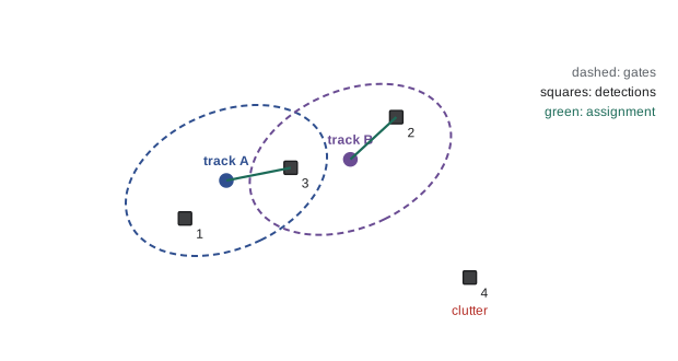
Worked problem
Global nearest neighbour
Two tracks A and B and two detections 1 and 2 have squared Mahalanobis distances A–1: 2.0, A–2: 3.0, B–1: 1.0, B–2: 6.0, all inside the gates. Compare nearest-neighbour and GNN assignments.
Show solution
- Nearest neighbour per track: A takes 1 (2.0), B takes 1 (1.0): a conflict over detection 1.
- GNN options: {A–1, B–2} costs 2.0 + 6.0 = 8.0; {A–2, B–1} costs 3.0 + 1.0 = 4.0.
- Choose the lower total: A–2, B–1.
Answer: GNN assigns detection 2 to A and detection 1 to B, total cost 4.0. Greedy nearest neighbour would have given detection 1 to both tracks. Note that A does not get its individually closest detection; the joint assignment is what matters.
Estimation in manipulation
Manipulation adds its own estimation problems. Before grasping, the robot estimates object pose from vision or depth, often with an ICP refinement and a covariance used to choose a grasp robust to the remaining error. During grasping and assembly, vision is often blocked by the gripper itself, so the estimate must be carried by other sensors: joint encoders give the gripper pose through forward kinematics, a wrist force-torque sensor indicates contact, and tactile sensors indicate where the object sits in the hand. A filter can fuse these, for example estimating the position of a peg in the gripper from tactile images, or detecting contact state (free, in contact, sliding, jammed) with a discrete Bayes filter over contact modes, which is the histogram filter of lesson 2 applied to an abstract state. Calibration is itself estimation: hand-eye calibration, which finds the transform between the camera and the gripper, is solved as a least-squares problem over many observed poses of a calibration target, and errors in it appear directly as errors in every grasp.
Worked problem
Is the pose good enough for insertion?
A vision system estimates a hole position with standard deviation 0.3 mm in each horizontal direction, independently. A peg has 0.5 mm radial clearance. Treating the 2-D position error as circular Gaussian, what is the probability that the error exceeds the clearance?
Show solution
- For a circular 2-D Gaussian, the radial error follows a Rayleigh distribution: \( P(r > c) = e^{-c^2/(2\sigma^2)} \).
- \( c^2/(2\sigma^2) = 0.25/0.18 = 1.389 \).
- \( P = e^{-1.389} = 0.249 \).
Answer: About a 25 % chance that the error exceeds the clearance, far too high for reliable insertion. The robot should improve the estimate (a closer camera, a larger target or several averaged images) or use a compliant strategy such as spiral search or impedance control from ROB-300 to absorb the remaining error.
Common mistakes
MistakeForgetting the reflection check in SVD alignment
InsteadInclude the determinant term so the result is a proper rotation.
MistakeRunning ICP from a poor initial guess
InsteadInitialize from features, a coarse search or a previous estimate.
MistakeAssigning detections greedily track by track
InsteadUse a global assignment such as the Hungarian algorithm when gates overlap.
MistakeConfirming tracks on a single detection
InsteadUse M-of-N confirmation to suppress tracks started by clutter.
MistakeExpressing rotation covariance in Euler angles
InsteadUse a small rotation-error vector about the estimate.
Summary and key terms
- With known correspondences, the SVD-based Kabsch method gives the optimal rotation and translation between point sets.
- ICP alternates nearest-point matching and alignment, and needs a good initial guess.
- Pose accuracy improves with point spread; angular error scales inversely with object size.
- Pose covariance can be estimated from residual Jacobians or by Monte Carlo, with rotations as small error vectors.
- Multi-target tracking runs a filter per track with prediction, association, update and track management.
- Gating limits candidates; global nearest neighbour solves the assignment jointly; JPDA and MHT avoid hard commitments.
- Manipulation fuses vision, kinematics, force and touch, and relies on calibration estimated by least squares.
- Kabsch method
- An SVD-based solution for the rotation and translation aligning two point sets.
- Iterative closest point
- An algorithm alternating nearest-point matching and alignment.
- Perspective-n-point
- Estimating camera pose from 2-D images of known 3-D points.
- Track
- A filter estimating the state of one target over time.
- Data association
- Deciding which measurements belong to which targets or to clutter.
- Global nearest neighbour
- The minimum-total-cost one-to-one assignment of detections to tracks.
- Hungarian algorithm
- An efficient method for solving assignment problems.
- JPDA
- Joint probabilistic data association, which weights all gated detections by their probabilities.
- Multiple hypothesis tracking
- Tracking that keeps several alternative association histories.
- M-of-N rule
- Confirming a track when it is detected in at least M of N frames.
Practice problems
Work each problem on paper first, then reveal the answer to check.
Model centroid (1, 1), measured centroid (4, 3), R = I. Find t.
Show answer
(3, 2).
Why does ICP need a good initial guess?
Show answer
Nearest-point matches from a poor guess can converge to a wrong alignment.
Point noise fixed, object twice as large. Effect on angular error?
Show answer
About halved.
Squared distances A–1: 4, A–2: 1, B–1: 2, B–2: 5. GNN assignment?
Show answer
A–2, B–1 (total 3).
Which method updates a track with a weighted mix of gated detections?
Show answer
JPDA.
False detection probability 0.2 per frame; 2-of-2 rule. Probability a false start confirms?
Show answer
0.2.
2-D circular Gaussian σ = 1 mm. Probability radial error exceeds 2 mm?
Show answer
\( e^{-2} = 0.135 \).
What algorithm finds pose from an AprilTag image?
Show answer
Perspective-n-point.
What discrete filter can track contact modes?
Show answer
A histogram (discrete Bayes) filter.
What calibration links the camera to the gripper?
Show answer
Hand-eye calibration.
Lesson quiz · 5 questions
Score 60% or more to complete this lesson.
Create a free account to save your progress, take quizzes and earn a certificate.