Motion models

The prediction step of the Bayes filter needs a motion model, the conditional distribution \( p(x_t \mid x_{t-1}, u_t) \) that says where the robot is likely to be after applying a control from a known starting pose. A deterministic kinematic model, such as the differential-drive equations from ROB-210, gives only the single pose the robot would reach if everything were perfect. A probabilistic motion model adds the uncertainty: wheel slip, uneven floors, encoder quantization and imperfect calibration. This lesson develops the two motion models used most in mobile robotics, the odometry model and the velocity model, shows how to sample from them and how to propagate a Gaussian through them, and explains why their uncertainty takes the curved 'banana' shape that motivates nonlinear filters later in the course.

Kinematics review for a planar robot

A planar mobile robot has pose \( \mathbf{x} = [x, y, \theta]^{\mathsf{T}} \): a position in the world frame and a heading measured anticlockwise from the x axis. A differential-drive robot with wheel radius r and track width b, whose wheels turn through small angles \( \Delta\phi_R \) and \( \Delta\phi_L \), moves forward by \( \Delta s = r(\Delta\phi_R + \Delta\phi_L)/2 \) and turns by \( \Delta\theta = r(\Delta\phi_R - \Delta\phi_L)/b \). For small steps, the pose update is

Using the midpoint heading \( \theta_{t-1} + \Delta\theta/2 \) is a second-order approximation of the arc the robot follows, accurate when each step is short. This deterministic model is the mean of the probabilistic motion model; the rest of the lesson is about the spread around it.

The odometry motion model

Most wheeled robots estimate their own motion by integrating wheel encoders, producing an odometry pose that drifts but is smooth and available at high rate. The odometry motion model treats the change in odometry between two times as the control. The relative motion from odometry pose \( \bar{\mathbf{x}}_{t-1} \) to \( \bar{\mathbf{x}}_t \) is decomposed into three steps: an initial rotation \( \delta_{rot1} \), a straight translation \( \delta_{trans} \) and a final rotation \( \delta_{rot2} \):

Each of the three is then assumed to be corrupted by independent zero-mean noise whose variance grows with the size of the motion. A common form, from Thrun, Burgard and Fox's Probabilistic Robotics, uses four parameters \( \alpha_1 \) to \( \alpha_4 \):

\( \alpha_1 \) sets how much rotation error comes from rotating, \( \alpha_2 \) how much rotation error comes from translating, \( \alpha_3 \) how much translation error comes from translating, and \( \alpha_4 \) how much translation error comes from rotating. Because the noise is applied to the motion rather than to the pose directly, the model naturally captures that driving farther or turning more produces more error. The odometry model is used in most particle-filter localization packages, including the widely used AMCL in ROS, whose parameters are named after these α values.

The velocity motion model

When a robot's controller commands a forward speed v and a turn rate ω, it is natural to model motion directly in those terms. With v and ω held constant over a step of length Δt, the robot follows a circular arc of radius \( v/\omega \), and the exact pose update is

with \( \theta_t = \theta_{t-1} + \omega\Delta t \). When ω is near zero the formula becomes numerically unstable and is replaced by straight-line motion, \( x_t = x_{t-1} + v\Delta t\cos\theta_{t-1} \). The probabilistic version adds noise to the commanded velocities, with variances that grow with speed, for example \( \sigma_v^2 = \alpha_1v^2 + \alpha_2\omega^2 \). The velocity model is preferred when odometry is unavailable, such as for a model-based prediction inside a planner, or for vehicles without wheel encoders where the commands are the best information about motion. The odometry model is usually more accurate when encoders exist, because it uses what the wheels actually did rather than what they were told to do.

Sampling from a motion model

Particle filters (lesson 8) never need to evaluate the motion model's density; they only need to draw samples from it. Sampling is straightforward: draw a noisy version of each motion component and apply the deterministic kinematics. For the odometry model, draw \( \hat{\delta}_{rot1} = \delta_{rot1} + \varepsilon_1 \), \( \hat{\delta}_{trans} = \delta_{trans} + \varepsilon_2 \) and \( \hat{\delta}_{rot2} = \delta_{rot2} + \varepsilon_3 \), with each ε drawn from a zero-mean Gaussian of the variance given above, then compute

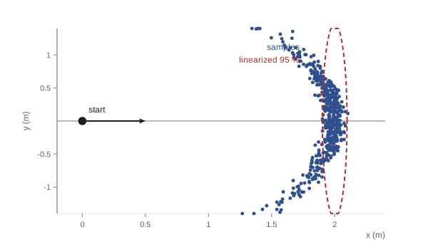
Repeating this many times from the same start produces a cloud of possible end poses. For straight driving with noticeable heading noise, the cloud is not an ellipse but a crescent, the banana distribution: the robot ends at roughly the same distance from the start, but spread along an arc, because a heading error rotates the end point around the start rather than pushing it sideways in a straight line.

Propagating a Gaussian through motion

Gaussian filters need the motion model in a different form: how does a Gaussian belief over the previous pose, with mean μ and covariance Σ, map to a Gaussian over the new pose? For a nonlinear motion function \( \mathbf{x}_t = g(\mathbf{x}_{t-1}, \mathbf{u}_t) + \text{noise} \), the standard approach linearizes g around the mean with its Jacobians. With \( \mathbf{G} = \partial g/\partial\mathbf{x} \) and \( \mathbf{V} = \partial g/\partial\mathbf{u} \), and control-noise covariance M,

For the simple model \( x_t = x + d\cos\theta,\ y_t = y + d\sin\theta,\ \theta_t = \theta + \delta \) with controls d and δ,

The term \( \mathbf{G}\boldsymbol{\Sigma}\mathbf{G}^{\mathsf{T}} \) moves and reshapes the old uncertainty, and the entries \( -d\sin\theta \) and \( d\cos\theta \) are what couple heading error into position error: the farther the robot drives, the more a heading error turns into sideways error. The term \( \mathbf{V}\mathbf{M}\mathbf{V}^{\mathsf{T}} \) adds the new noise from this step. This is exactly the prediction step of the extended Kalman filter in lesson 6.

import numpy as np
rng = np.random.default_rng(3)
N, d = 2000, 2.0
sig_th0, sig_d, sig_rot = 0.15, 0.04, 0.05          # initial heading, translation, rotation noise
th0 = rng.normal(0, sig_th0, N)                      # uncertain starting heading
dd = d + rng.normal(0, sig_d, N)
x = dd*np.cos(th0); y = dd*np.sin(th0); th = th0 + rng.normal(0, sig_rot, N)
print(f"sample mean x = {x.mean():.3f} m (linearized mean = {d:.3f} m)")
print(f"sample std  y = {y.std():.3f} m (linearized = {d*sig_th0:.3f} m)")
# linearized covariance at the mean heading 0
G = np.array([[1, 0, 0], [0, 1, d], [0, 0, 1]]); S0 = np.diag([0, 0, sig_th0**2])
V = np.array([[1, 0], [0, 0], [0, 1]]); M = np.diag([sig_d**2, sig_rot**2])
S = G @ S0 @ G.T + V @ M @ V.T
print("linearized covariance diag:", np.round(np.diag(S), 4))
print("sample covariance diag:    ", np.round(np.var(np.c_[x, y, th], axis=0), 4))

sample mean x = 1.978 m (linearized mean = 2.000 m)
sample std  y = 0.295 m (linearized = 0.300 m)
linearized covariance diag: [0.0016 0.09   0.025 ]
sample covariance diag:     [0.0025 0.0868 0.0244]

The linearized prediction gets the lateral spread almost right but misses two things. The sample mean in x is a few centimetres short of 2 m, because every heading error, positive or negative, shortens the forward distance by \( d(1 - \cos\theta) \); a linearized model, symmetric by construction, cannot see this bias. And the linearized x variance contains only the translation noise, while the samples show extra x spread from the curvature. With small heading uncertainty these errors are negligible and the extended Kalman filter works well; with large heading uncertainty, such as after a long stretch without a heading reference, the banana becomes pronounced and filters that can represent it, the unscented Kalman filter and particle filters, do better.

Calibrating motion models

The α parameters or velocity noise variances are rarely known from first principles; they are calibrated. A common procedure drives the robot repeatedly along known paths, such as straight 5 m runs and on-the-spot rotations of 360°, measures the true end poses with an external system (a motion-capture system, a total station or careful tape measurement), and fits the noise parameters so that the predicted spread matches the observed spread. Systematic errors should be removed first: an incorrect wheel radius or track width produces a consistent bias that no zero-mean noise model can represent, so these are calibrated by methods such as the UMBmark square-path test before noise parameters are fitted. A good rule is to err on the side of slightly too much noise, because an overconfident motion model makes the filter ignore measurements that would correct it, while a slightly pessimistic one only costs a little accuracy.