Oscillators revisited: anharmonic and nonlinear motion

PHYS-230 developed the linear oscillator in depth: the free, damped and driven cases, resonance and the quality factor, coupled oscillators and normal modes. All of that rested on a restoring force exactly proportional to displacement. Lesson 4 showed that this is only an approximation, valid for small displacements, and that a real pendulum's period grows with amplitude. This lesson asks what happens when the nonlinear terms matter. The answers include frequencies that shift with amplitude, new harmonics, resonance curves that bend over and jump, oscillations that a child on a swing pumps up by standing and crouching, and oscillations that sustain themselves at a fixed size whatever the starting conditions.

The Duffing equation

The simplest nonlinear correction to a symmetric spring adds a cubic term to the restoring force. In dimensionless form, with time measured in units of \(1/\omega_0\),

This is the Duffing equation, studied by the German engineer Georg Duffing in 1918 for the vibrations of machinery. With \(\beta > 0\) the spring stiffens as it stretches (a hardening spring); with \(\beta < 0\) it softens. The pendulum is a softening case: expanding \(\sin\theta \approx \theta - \theta^3/6\) gives \(\beta = -1/6\). A taut string vibrating with large amplitude, a beam clamped at both ends, and the bonds in a crystal are hardening. The potential is \(U = \tfrac12x^2 + \tfrac14\beta x^4\), so by lesson 4 the motion is periodic for any energy when \(\beta > 0\), with a period that depends on the amplitude.

Frequency shift by perturbation theory

For small \(\beta\) we expect the solution to be close to \(x = A\cos t\). The naive approach is to write \(x = x_0 + \beta x_1 + \cdots\) and solve order by order. At first order this gives \(\ddot x_1 + x_1 = -A^3\cos^3 t\). Using \(\cos^3 t = \tfrac34\cos t + \tfrac14\cos 3t\), the right-hand side contains a term at the natural frequency, which drives \(x_1\) at resonance and produces a secular term \(t\sin t\) that grows without bound. The true solution is bounded, so the expansion has failed. The trouble is that the frequency itself changes with amplitude, and a small error in frequency produces a phase error that grows linearly with time.

The method of Anders Lindstedt (1882), made rigorous by Poincaré, fixes this by expanding the frequency as well. Write \(\tau = \omega t\) with \(\omega = 1 + \beta\omega_1 + \cdots\) and \(x = x_0(\tau) + \beta x_1(\tau) + \cdots\). The equation becomes \(\omega^2x'' + x + \beta x^3 = 0\), where primes denote \(d/d\tau\). At zeroth order \(x_0 = A\cos\tau\). At first order,

The resonant \(\cos\tau\) term must vanish for \(x_1\) to stay bounded, which fixes \(\omega_1 = \tfrac38A^2\). The remaining equation gives a third harmonic, \(x_1 = \tfrac1{32}A^3(\cos3\tau - \cos\tau)\) with the initial conditions \(x(0) = A\), \(\dot x(0) = 0\). So to first order

A hardening spring oscillates faster at large amplitude and a softening spring slower. For the pendulum, \(\beta = -1/6\) gives \(\omega \approx 1 - \theta_0^2/16\), which matches the series \(T/T_0 \approx 1 + \theta_0^2/16\) of lesson 4. The third harmonic means the motion is no longer a pure sinusoid: a nonlinear oscillator driven at frequency \(\omega\) radiates at \(3\omega\) as well, which is the principle behind frequency tripling in nonlinear optics and the distortion of a loudspeaker driven too hard.

Checking the perturbation result numerically

The first part of the program integrates the free Duffing oscillator with RK4, measures the period from successive maxima, and compares the frequency with Lindstedt's formula for three amplitudes. The second part adds damping and a periodic drive and sweeps the driving frequency, first upward and then downward, recording the steady-state amplitude at each step.

import math

def rk4(f, t, y, dt):
    k1 = f(t, y); k2 = f(t + dt / 2, [a + dt / 2 * b for a, b in zip(y, k1)])
    k3 = f(t + dt / 2, [a + dt / 2 * b for a, b in zip(y, k2)]); k4 = f(t + dt, [a + dt * b for a, b in zip(y, k3)])
    return [a + dt / 6 * (b1 + 2 * b2 + 2 * b3 + b4) for a, b1, b2, b3, b4 in zip(y, k1, k2, k3, k4)]

# 1. Free Duffing oscillator x'' + x + beta x^3 = 0: measured frequency versus Lindstedt's 1 + 3 beta A^2 / 8
beta = 0.5
for A in (0.2, 0.5, 1.0):
    t, y, dt, ups = 0.0, [A, 0.0], 0.001, []
    f = lambda t, s: [s[1], -s[0] - beta * s[0] ** 3]
    while len(ups) < 3:
        new = rk4(f, t, y, dt)
        if y[1] > 0 >= new[1]:                       # velocity crosses zero downward: a maximum of x
            ups.append(t + dt * y[1] / (y[1] - new[1]))
        y, t = new, t + dt
    w = 2 * math.pi / (ups[2] - ups[1])
    print(f"A = {A:.1f}: omega = {w:.5f}, Lindstedt {1 + 3 * beta * A * A / 8:.5f}")

# 2. Driven, damped Duffing: x'' + gamma x' + x + beta x^3 = F cos(w t). Sweep w up, then down.
gamma, beta, F = 0.1, 0.2, 0.25
def steady_amp(w, y):
    f = lambda t, s: [s[1], F * math.cos(w * t) - gamma * s[1] - s[0] - beta * s[0] ** 3]
    T = 2 * math.pi / w; n = 200; dt = T / n; t = 0.0
    for _ in range(60 * n):                          # let transients die
        y = rk4(f, t, y, dt); t += dt
    amp = 0.0
    for _ in range(4 * n):
        y = rk4(f, t, y, dt); t += dt; amp = max(amp, abs(y[0]))
    return amp, y
ws = [0.8 + 0.05 * i for i in range(15)]
up, y = [], [0.0, 0.0]
for w in ws:
    a, y = steady_amp(w, y); up.append(a)
down, y = [], [0.0, 0.0]
for w in reversed(ws):
    a, y = steady_amp(w, y); down.append(a)
down.reverse()
print("  w     sweep up   sweep down")
for w, a, b in zip(ws, up, down):
    flag = "  <- two stable states" if abs(a - b) > 0.2 else ""
    print(f"{w:5.2f}   {a:7.3f}    {b:7.3f}{flag}")

A = 0.2: omega = 1.00747, Lindstedt 1.00750
A = 0.5: omega = 1.04566, Lindstedt 1.04688
A = 1.0: omega = 1.17078, Lindstedt 1.18750
  w     sweep up   sweep down
 0.80     0.596      0.596
 0.85     0.697      0.697
 0.90     0.824      0.824
 0.95     0.977      0.977
 1.00     1.147      1.147
 1.05     1.326      1.326
 1.10     1.507      1.507
 1.15     1.683      1.683
 1.20     1.851      0.627  <- two stable states
 1.25     1.993      0.459  <- two stable states
 1.30     0.367      0.367
 1.35     0.305      0.305
 1.40     0.260      0.260
 1.45     0.226      0.226
 1.50     0.200      0.200

At \(A = 0.2\) the measured frequency 1.00747 agrees with the first-order formula to within \(3\times10^{-5}\). At \(A = 1\) the formula overshoots by 1.4%, because the next correction, of order \(\beta^2A^4\), is no longer negligible with \(\beta A^2 = 0.5\). The perturbation method is reliable when the nonlinear term is small compared with the linear one, and degrades gracefully beyond that.

The driven Duffing oscillator

Add damping and a periodic force: \(\ddot x + \gamma\dot x + x + \beta x^3 = F\cos\omega t\). For a linear oscillator (\(\beta = 0\)), PHYS-230 showed that the steady-state amplitude traces a single symmetric resonance peak at \(\omega \approx 1\). For the Duffing oscillator, try \(x \approx A\cos(\omega t - \phi)\) and keep only the terms at frequency \(\omega\), using \(\cos^3 = \tfrac34\cos + \tfrac14\cos3\). This harmonic-balance approximation gives

Compare the linear result \(\big[(1 - \omega^2)^2 + \gamma^2\omega^2\big]A^2 = F^2\). The nonlinearity has replaced the natural frequency 1 by the amplitude-dependent frequency \(\sqrt{1 + \tfrac34\beta A^2}\), the same backbone curve found by perturbation theory. Since large amplitudes have a higher natural frequency for \(\beta > 0\), the resonance peak leans toward higher frequencies. If it leans far enough, the curve folds back on itself, and for a range of driving frequencies there are three possible steady amplitudes. The middle one is unstable; the outer two are both stable.

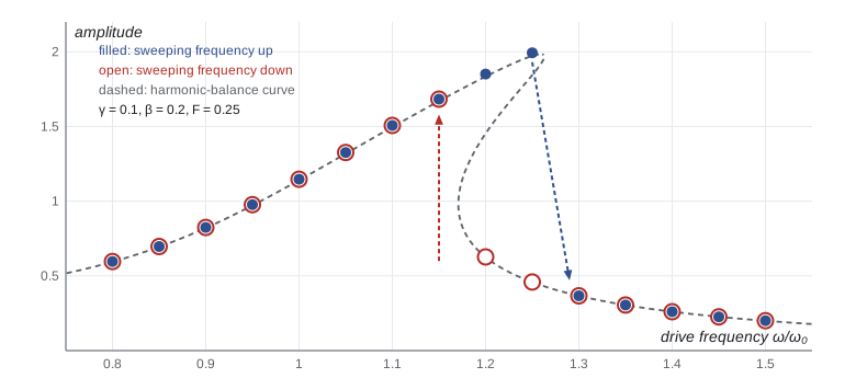
The frequency sweep in the program shows the consequence. Sweeping upward, the oscillator rides the upper branch to an amplitude of 1.99 at \(\omega = 1.25\), then at 1.30 falls abruptly to 0.37. Sweeping downward, it stays on the lower branch until 1.20, where the amplitude is only 0.63, and only at 1.15 jumps back up. At 1.20 and 1.25 two different stable oscillations exist for exactly the same drive, and which one you see depends on the history. This hysteresis, with sudden jumps at the edges of the fold, is a hallmark of nonlinear resonance. It appears in micromechanical resonators used as sensors, in the rolling of ships in waves, in the vibration of turbine blades, and in the response of some bridges to wind and footfall.

Parametric resonance

A child on a swing does not need anyone to push. By standing up as the swing passes through the bottom and crouching at the ends, the child periodically changes the effective length of the pendulum, and the amplitude grows. This is parametric excitation: a parameter of the system, not an external force, varies in time. The model equation is Mathieu's equation (Émile Mathieu, 1868),

The striking result is that the strongest instability occurs when \(\Omega = 2\omega_0\): the parameter must be modulated at twice the natural frequency, so that it changes twice per cycle of the motion. With a small modulation depth \(h\), the amplitude grows exponentially, at a rate of about \(h\omega_0/4\), when \(|\Omega - 2\omega_0| < h\omega_0/2\). Weaker instabilities occur near \(\Omega = 2\omega_0/n\) for every integer \(n\). Because the growth is exponential rather than linear, parametric resonance needs no matching external force, only the right timing. Michael Faraday saw it in 1831 when a vertically shaken dish of liquid produced surface waves at half the shaking frequency, and engineers meet it whenever a structure's stiffness varies periodically, as in a rotating shaft that is stiffer in one direction than another.

Self-sustained oscillations

A violin string bowed steadily, a heart beating, a clock escapement and an electronic oscillator all settle into an oscillation of a definite amplitude, whatever their starting state. A linear system cannot do this: its free oscillations either decay, grow or keep whatever amplitude they began with. The standard model, introduced by the Dutch engineer Balthasar van der Pol in the 1920s for vacuum-tube circuits, has damping that depends on amplitude:

For small \(|x|\) the damping coefficient \(-\mu(1 - x^2)\) is negative, so energy is fed in and the oscillation grows. For large \(|x|\) it is positive, so energy is removed. The balance is struck on a closed curve in the phase plane, the limit cycle, which every trajectory approaches from inside and outside. For small \(\mu\) the limit cycle is nearly a circle of radius 2. Averaging the energy input over a cycle of \(x = A\cos t\) shows why: the work done per cycle is \(\mu\pi A^2(1 - A^2/4)\), which vanishes at \(A = 2\). For large \(\mu\) the oscillation becomes a relaxation oscillation, with slow build-ups and sudden snaps, much like a dripping tap or the stick-slip of a squeaking door.

Why nonlinearity matters

Linear systems obey superposition: the response to two inputs is the sum of the responses to each, and doubling the input doubles the output. Nonlinear systems do not, which is why they can generate new frequencies, settle at amplitudes fixed by the system rather than the input, and remember their history. These features are often unwanted (distortion, sudden jumps in vibration) and sometimes exploited (frequency multipliers, clocks, mechanical memory elements). In lesson 12 we push nonlinearity further and find that a driven, damped, nonlinear oscillator can lose all regularity and become chaotic.