Capstone: chaos and the limits of prediction

This course began with Laplace's claim that a mind knowing every position and velocity could predict the whole future. It ends by examining when that claim fails in practice. Every system in this lesson obeys Newton's laws exactly, with no randomness anywhere. Yet a double pendulum, a driven pendulum, three gravitating bodies and even a one-line formula iterated on a calculator can produce behaviour that is impossible to forecast beyond a short horizon. The capstone draws on almost every earlier lesson: the state space of lesson 1, the potentials and separatrices of lesson 4, the nonlinear oscillators of lesson 5, the orbits of lessons 7 and 8, and the numerical methods used throughout.

Sensitive dependence on initial conditions

Two starting states that differ by a tiny amount \(\delta_0\) follow nearby paths at first. In a regular system the separation grows slowly, typically in proportion to time; two pendulums with slightly different amplitudes drift out of phase because their periods differ a little. In a chaotic system the separation grows exponentially,

where \(\lambda > 0\) is the largest Lyapunov exponent, named for the Russian mathematician Aleksandr Lyapunov, whose 1892 thesis founded the theory of stability. Exponential growth is relentless. If \(\lambda = 1\) per second and you measure the starting state to one part in a billion, the prediction is worthless after \(\ln(10^9) \approx 21\) seconds. Improving the measurement a thousandfold, to one part in a trillion, buys only another 7 seconds. The prediction horizon grows only as the logarithm of the precision. This is the real meaning of the butterfly effect, a phrase that comes from the title of a 1972 talk by Edward Lorenz.

The separation cannot grow forever: once it is as large as the region the motion is confined to, the two paths are simply unrelated. Chaos therefore needs two ingredients that seem contradictory: stretching, which separates nearby states, and folding, which keeps the motion bounded. Picture kneading dough. Two raisins that start close are pulled apart by each stretch and brought back near other raisins by each fold, until their positions are effectively scrambled.

The logistic map

The cleanest example of chaos is not a mechanical system at all but a single equation, the logistic map, made famous by the biologist Robert May in 1976 as a model of population growth:

Here \(x_n\) is a population in year \(n\) as a fraction of its maximum. Each year it grows by the factor \(r\), but crowding cuts the growth by \(1 - x_n\). For \(r < 3\) the population settles to a fixed point \(x^* = 1 - 1/r\). At \(r = 3\) the fixed point becomes unstable and the population alternates between two values: a period-two cycle. At \(r \approx 3.449\) that cycle becomes unstable and period four appears, then period eight at 3.544, and so on, with the doublings coming faster and faster until they accumulate at \(r_\infty \approx 3.5699\). Beyond that point the population wanders irregularly and never repeats.

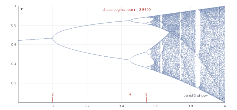
The program finds the doubling points numerically and measures the Lyapunov exponent, the average of \(\ln|f'(x_n)| = \ln|r(1 - 2x_n)|\) along the orbit, which is the average rate at which nearby orbits separate per step.

import math

# 1. The logistic map x -> r x (1 - x): period doubling, Feigenbaum's ratio and the Lyapunov exponent
def attractor(r, n_skip=2000, n_keep=256):
    x = 0.4
    for _ in range(n_skip): x = r * x * (1 - x)
    pts = set()
    for _ in range(n_keep):
        x = r * x * (1 - x); pts.add(round(x, 6))
    return len(pts)

def lyapunov(r, n=20000):
    x, s = 0.4, 0.0
    for _ in range(500): x = r * x * (1 - x)
    for _ in range(n):
        x = r * x * (1 - x); s += math.log(abs(r * (1 - 2 * x)))
    return s / n

for r in (2.8, 3.2, 3.5, 3.55, 3.7, 3.83, 4.0):
    print(f"r = {r:4.2f}: {attractor(r):3d} distinct points, Lyapunov exponent {lyapunov(r):+.3f}")

def doubling_point(target, lo, hi):
    # smallest r at which the attractor has at least `target` points (bisection)
    for _ in range(40):
        mid = 0.5 * (lo + hi)
        if attractor(mid, 20000, 512) >= target: hi = mid
        else: lo = mid
    return hi
rs = [doubling_point(2 ** k, 2.9, 3.57) for k in range(1, 6)]
print("period-doubling points:", ", ".join(f"{r:.5f}" for r in rs))
print("ratios of successive gaps:", ", ".join(f"{(rs[i] - rs[i - 1]) / (rs[i + 1] - rs[i]):.3f}" for i in range(1, 4)))

# 2. Double pendulum (equal masses and lengths, g = L = 1): two starts 1e-9 rad apart
def deriv(s):
    t1, t2, w1, w2 = s
    d = t1 - t2
    den = 3 - math.cos(2 * d)
    a1 = (-3 * math.sin(t1) - math.sin(t1 - 2 * t2) - 2 * math.sin(d) * (w2 * w2 + w1 * w1 * math.cos(d))) / den
    a2 = (2 * math.sin(d) * (2 * w1 * w1 + 2 * math.cos(t1) + w2 * w2 * math.cos(d))) / den
    return [w1, w2, a1, a2]
def rk4(s, dt):
    k1 = deriv(s); k2 = deriv([a + dt / 2 * b for a, b in zip(s, k1)])
    k3 = deriv([a + dt / 2 * b for a, b in zip(s, k2)]); k4 = deriv([a + dt * b for a, b in zip(s, k3)])
    return [a + dt / 6 * (p + 2 * q + 2 * r + w) for a, p, q, r, w in zip(s, k1, k2, k3, k4)]
energy = lambda s: (s[2] ** 2 + 0.5 * s[3] ** 2 + s[2] * s[3] * math.cos(s[0] - s[1])) - 2 * math.cos(s[0]) - math.cos(s[1])
for start, label in ((math.radians(10), "small swing (10 deg)"), (math.radians(120), "large swing (120 deg)")):
    a = [start, start, 0.0, 0.0]; b = [start + 1e-9, start, 0.0, 0.0]
    E0, dt, logs = energy(a), 0.002, []
    for step in range(1, 20001):
        a, b = rk4(a, dt), rk4(b, dt)
        if step % 5000 == 0:
            sep = math.sqrt(sum((x - y) ** 2 for x, y in zip(a, b)))
            logs.append((step * dt, sep))
    rate = math.log(logs[1][1] / logs[0][1]) / (logs[1][0] - logs[0][0])
    print(f"{label}: separation at t = 10, 20, 30, 40: " + ", ".join(f"{s:.1e}" for _, s in logs)
          + f"; growth rate {rate:.2f} per unit time; energy error {abs(energy(a) - E0):.1e}")

r = 2.80:   1 distinct points, Lyapunov exponent -0.223
r = 3.20:   2 distinct points, Lyapunov exponent -0.916
r = 3.50:   4 distinct points, Lyapunov exponent -0.873
r = 3.55:   8 distinct points, Lyapunov exponent -0.100
r = 3.70: 255 distinct points, Lyapunov exponent +0.356
r = 3.83:   3 distinct points, Lyapunov exponent -0.370
r = 4.00: 256 distinct points, Lyapunov exponent +0.693
period-doubling points: 2.99948, 3.44931, 3.54403, 3.56438, 3.56875
ratios of successive gaps: 4.749, 4.653, 4.657
small swing (10 deg): separation at t = 10, 20, 30, 40: 1.3e-09, 1.7e-09, 1.6e-09, 1.6e-09; growth rate 0.03 per unit time; energy error 1.3e-15
large swing (120 deg): separation at t = 10, 20, 30, 40: 1.2e-08, 1.0e-06, 3.8e-05, 6.6e-02; growth rate 0.44 per unit time; energy error 2.4e-10

The Lyapunov exponent is negative wherever the orbit settles into a cycle and positive in the chaotic regions: \(+0.356\) at \(r = 3.7\) and exactly \(\ln 2 = 0.693\) at \(r = 4\), where the map can be solved by a change of variables and is equivalent to doubling an angle. At \(r = 3.83\) the motion has returned to order, a stable period-3 cycle inside the chaotic region. The ratios of successive gaps between doubling points come out as 4.749, 4.653 and 4.657, approaching a limit. (The first doubling is at exactly 3; the program reports 2.9995 because convergence is very slow right at a bifurcation.)

In 1978 Mitchell Feigenbaum, working at Los Alamos with a programmable calculator, discovered that this limit, \(\delta = 4.6692\ldots\), is the same for every smooth map with a single hump, and later experiments found it in dripping taps, convecting liquid helium and electronic circuits. Universality of this kind means that the route to chaos does not depend on the details of the system, much as the critical exponents of phase transitions do not.

The driven damped pendulum

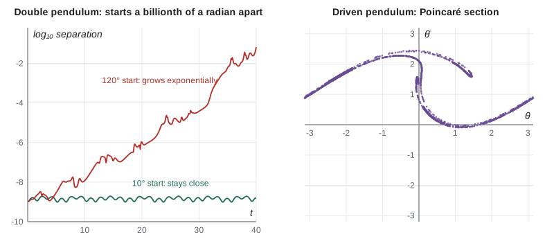
A pendulum with damping and a periodic driving torque obeys \(\ddot\theta + \dot\theta/Q + \sin\theta = F\cos\omega_dt\), in units where the natural frequency is 1. Three ingredients make chaos possible: the nonlinearity of \(\sin\theta\), the drive, and the fact that the state space \((\theta, \dot\theta, \text{phase of the drive})\) is three-dimensional. (In two dimensions, the Poincaré–Bendixson theorem forbids chaos: trajectories cannot cross, so they can only settle on fixed points or closed loops.) For weak driving the pendulum oscillates in step with the drive. As \(F\) increases, it goes through period doubling much like the logistic map, and for \(Q = 2\), \(\omega_d = 2/3\) and \(F = 1.5\), a classic set of values studied by Gregory Baker and Jerry Gollub, it swings irregularly, sometimes going over the top one way, sometimes the other, never repeating.

To see the structure in such motion, Poincaré introduced a section: instead of drawing the whole trajectory, mark the state once per drive period. A periodic motion gives a single point, or a few. A chaotic motion gives a set of points that never repeats but is not random either; it lies on a strange attractor with an intricate folded structure that looks similar at every magnification, a fractal. The right panel of the figure shows the Poincaré section of the driven pendulum after 2200 drive periods.

The double pendulum

A double pendulum, one pendulum hanging from the bob of another, is the classic tabletop demonstration of chaos. It has no damping and no drive, so its energy is conserved, yet for large swings its motion is chaotic. The program integrates two copies with RK4, starting one a billionth of a radian away from the other, at a small amplitude (\(10^\circ\)) and a large one (\(120^\circ\)). At \(10^\circ\) the separation hardly grows: the motion is a combination of two normal modes, like the coupled oscillators of PHYS-230, and it is regular. At \(120^\circ\) the separation grows from \(10^{-8}\) to \(10^{-1}\) in 30 time units, an average rate of about 0.5 per unit time. For a pendulum with arms 1 m long the time unit is \(\sqrt{\ell/g} = 0.32\ \mathrm{s}\), so the separation doubles roughly every half second, and a measurement accurate to a billionth of a radian is useless after about 15 seconds. The energy error of \(2\times10^{-10}\) shows that the divergence is real, not a numerical artifact.

Not every starting state of the double pendulum is chaotic. Low-energy motions are regular, and even at higher energies islands of regular motion survive amid the chaotic sea. The Kolmogorov–Arnold–Moser theorem, developed between 1954 and 1963, explains why: when a regular system is gently perturbed, most of its regular motions survive in distorted form, and chaos first appears in thin layers around the separatrices, exactly where lesson 4 showed motion to be most delicate. As the perturbation grows, the chaotic layers widen and merge.

The three-body problem and the solar system

Newton solved the two-body problem completely in lessons 7 and 8. Adding a third body changes everything. In 1887 King Oscar II of Sweden offered a prize for a proof that the solar system is stable. Henri Poincaré's winning memoir of 1890 contained an error, which he found after the prize was awarded; correcting it, he discovered that the three-body problem has solutions so tangled that, in his words, one is struck by the complexity of the figure that he did not even attempt to draw. This was the first glimpse of chaos. Special solutions exist (Euler's collinear and Lagrange's equilateral configurations of 1767 and 1772, where the James Webb Space Telescope now orbits near the Sun–Earth L2 point), but the general motion is chaotic.

Is the solar system itself chaotic? Numerical integrations by Jacques Laskar beginning in 1989 found that the inner planets have a Lyapunov time of about 5 million years: an error of 15 m in the Earth's position today grows to an error of the size of its orbit in about 100 million years. Over the Sun's remaining lifetime there is roughly a 1% chance that Mercury's orbit becomes eccentric enough to cross Venus's. The planets are not going to fly apart any time soon, but their precise positions millions of years from now are fundamentally unknowable.

What chaos means for prediction

Chaos does not make mechanics useless; it changes the questions. Over time scales much shorter than the Lyapunov time, deterministic prediction works, which is why spacecraft reach their targets and weather forecasts are good for several days. Over longer times we predict statistics instead: the average temperature of next January, the fraction of time a pendulum spends near the bottom, the probability that an asteroid's orbit will cross the Earth's. The same equations that make individual trajectories unpredictable often make long-run averages extremely reliable, which is the bridge from mechanics to the statistical mechanics of PHYS-361.

Looking back over the course

We started with Newton's laws as differential equations and the state of a system as a point in state space. We added drag and variable mass, then used energy to understand motion in a potential without solving for the time. We saw how nonlinearity bends resonance curves and creates limit cycles, developed the vector calculus of three-dimensional motion, and solved the central-force problem from Kepler's laws to Hohmann transfers to Rutherford's discovery of the nucleus. We learned to work in rotating frames and with rotating bodies. And we have now seen that the same deterministic laws can produce motion that is regular, quasi-regular or chaotic. PHYS-344 recasts all of this in the Lagrangian and Hamiltonian language that underlies quantum mechanics and modern dynamics, where symmetries and conservation laws take centre stage.