Fourier analysis, dispersion and wave packets

In 1807 Joseph Fourier presented a memoir on heat flow to the Paris Academy claiming that any function on an interval, even one with corners and jumps, can be written as a sum of sines and cosines. The examiners, who included Lagrange, were doubtful, and the work was published in full only in 1822 as The Analytical Theory of Heat. Fourier was essentially right, and his idea is now one of the most used tools in science and engineering. For waves it means that any disturbance can be analysed as a superposition of sinusoids, each of which we already understand. This lesson develops Fourier series and transforms, the trade-off between duration and bandwidth, the discrete Fourier transform that computers use, and then dispersion: what happens to a wave packet when sinusoids of different frequencies travel at different speeds. That leads to the group velocity, the speed at which energy and information actually travel.

Fourier series

A function \(f(t)\) with period \(T\) and angular frequency \(\omega_1 = 2\pi/T\) can be written

The coefficient formulas follow by multiplying the series by \(\cos m\omega_1t\) or \(\sin m\omega_1t\), integrating over a period, and using orthogonality: the integral of a product of two different harmonics over a period is zero, and the integral of a harmonic squared is \(T/2\). For any function that is piecewise smooth, Dirichlet proved in 1829 that the series converges to \(f(t)\) where \(f\) is continuous and to the midpoint of the jump where it is not. The complex form is often neater: \(f(t) = \sum_{n=-\infty}^{\infty} c_ne^{in\omega_1t}\) with \(c_n = \frac1T\int_0^T f(t)e^{-in\omega_1t}\,dt\).

Take the square wave equal to \(+1\) for \(0 < t < T/2\) and \(-1\) for \(T/2 < t < T\). It is odd, so all \(a_n = 0\), and

which is \(4/n\pi\) for odd \(n\) and zero for even \(n\). So

The coefficients fall only as \(1/n\), because the function has jumps; a function with corners but no jumps, like the plucked string of lesson 6, has coefficients falling as \(1/n^2\), and smoother functions converge faster still. Near a jump the partial sums overshoot. However many terms are kept, the first peak beside the jump exceeds the true value by about 9 parts in a hundred of the size of the jump; the overshoot narrows toward the jump but does not shrink. This is the Gibbs phenomenon, described by Henry Wilbraham in 1848 and by J. Willard Gibbs in 1898–99, and it is why sharp edges in images and audio processed with truncated Fourier series show ringing.

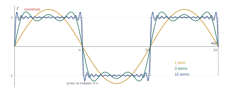
Energy is shared among the harmonics. Parseval's theorem states that the mean square of the function equals the sum of the mean squares of its harmonics, \(\frac1T\int_0^T f^2\,dt = \frac{a_0^2}{4} + \frac12\sum(a_n^2 + b_n^2)\). For the square wave the left side is 1, and the right side is \(\frac12\cdot\frac{16}{\pi^2}(1 + \frac19 + \frac1{25} + \cdots)\), which gives Euler's famous sum \(1 + \frac19 + \frac1{25} + \cdots = \pi^2/8\). For a sound wave Parseval says the power is the sum of the powers in each harmonic, which is what a spectrum analyser displays.

The Fourier transform

A pulse that happens once is not periodic. Let the period \(T\) grow without bound: the harmonics \(n\omega_1\) crowd together into a continuum, and the series becomes an integral,

\(F(\omega)\) is the spectrum of the pulse: how much of each frequency it contains. Two examples matter most. A Gaussian pulse \(f(t) = e^{-t^2/2\tau^2}\) has a Gaussian spectrum \(F(\omega) = \sqrt{2\pi}\,\tau\,e^{-\omega^2\tau^2/2}\), of width \(1/\tau\) in angular frequency. A finite wave train, \(\cos\omega_0t\) switched on for a duration \(\Delta t\), has a spectrum centred on \(\omega_0\) with width of order \(2\pi/\Delta t\). In both cases the product of the duration and the bandwidth is fixed: short pulses are broadband and narrow spectral lines require long wave trains. With rms widths the precise statement is

with equality for the Gaussian. This bandwidth theorem is pure mathematics, not physics, but it has physical consequences everywhere. It is why the resonance of lesson 3 with width \(\gamma\) rings for a time \(1/\gamma\); why a 10 fs laser pulse at 800 nm must contain wavelengths spread over about 100 nm; why a digital link that sends a billion pulses per second needs a gigahertz of bandwidth; and, multiplied by Planck's constant, why quantum mechanics has the energy-time uncertainty relation.

The discrete Fourier transform

A computer samples a signal at \(N\) equally spaced times \(t_j = j\Delta t\) and computes

the discrete Fourier transform. Component \(k\) corresponds to frequency \(k/(N\Delta t)\), so the frequency resolution is \(1/(N\Delta t)\), the reciprocal of the record length, another form of the bandwidth theorem. Sampling imposes a limit too. A sinusoid at frequency \(f\) and one at \(f + 1/\Delta t\) give identical samples, so frequencies above the Nyquist frequency \(f_s/2\), half the sampling rate, are indistinguishable from lower ones: they alias. Harry Nyquist identified the limit in 1928, and Claude Shannon's sampling theorem of 1949 showed that a signal containing no frequencies above \(f_s/2\) is completely determined by its samples. CD audio samples at 44.1 kHz so that the whole audible range up to about 20 kHz is captured. Computed directly, the transform takes about \(N^2\) operations; the fast Fourier transform published by James Cooley and John Tukey in 1965, anticipated by Gauss around 1805, takes about \(N\log_2N\), which turns a million-point transform from a trillion operations into twenty million.

Dispersion

On an ideal string every frequency travels at the same speed, so a pulse keeps its shape. In a dispersive medium the phase velocity \(\omega/k\) depends on frequency, and the components of a pulse drift apart. Examples are everywhere. Deep-water surface waves obey \(\omega = \sqrt{gk}\), so long waves outrun short ones. Light in glass has a refractive index that falls with wavelength, so blue travels more slowly than red, which is why prisms spread white light. A stiff piano string has \(\omega^2 = v^2k^2 + \beta k^4\), which makes its upper partials slightly sharp of true harmonics, a property tuners compensate for by stretching the octaves. And the electron gas in the ionosphere gives radio waves \(\omega^2 = \omega_p^2 + c^2k^2\), with no propagation at all below the plasma frequency \(\omega_p\).

Phase and group velocity

Superpose two waves of nearly equal wavenumber and frequency, \(k \pm \Delta k\) and \(\omega \pm \Delta\omega\):

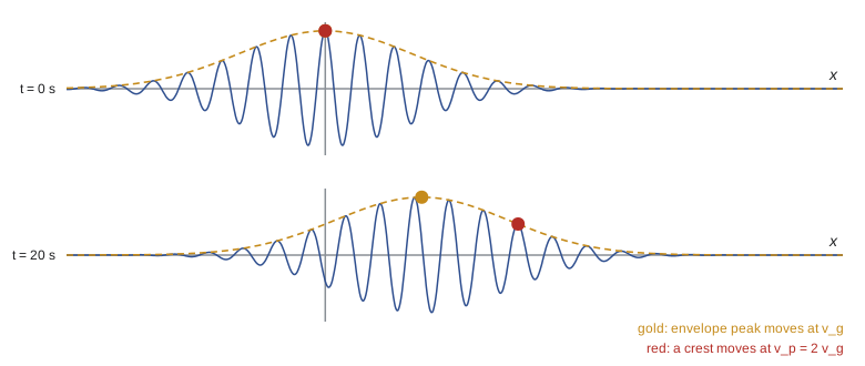
The fast factor is a carrier wave whose crests move at the phase velocity \(v_p = \omega/k\). The slow factor is an envelope, a pattern of beats in space, whose peaks move at \(\Delta\omega/\Delta k\). In the limit of a narrow band of wavenumbers this becomes the group velocity

A general packet \(\int A(k)e^{i(kx - \omega(k)t)}dk\) with \(A(k)\) peaked at \(k_0\) can be handled by expanding \(\omega(k) \approx \omega_0 + v_g(k - k_0)\): the integral becomes \(e^{i(k_0x - \omega_0t)}\) times a function of \(x - v_gt\) alone, so the envelope moves rigidly at \(v_g\) to first order. The second-order term \(\tfrac12\omega''(k - k_0)^2\) makes the envelope spread, which is group-velocity dispersion. Energy and information travel with the envelope, at the group velocity. For deep-water waves \(\omega = \sqrt{gk}\) gives \(v_g = \tfrac12\sqrt{g/k} = v_p/2\): watch the wake of a boat and you see individual crests appear at the back of a wave group, run forward through it and vanish at the front. For light in a medium of index \(n(\lambda)\), the group index is \(n_g = n - \lambda\,dn/d\lambda\), larger than \(n\) in normal dispersion, so pulses in an optical fibre travel more slowly than the phase velocity \(c/n\).

The phase velocity can exceed \(c\), for example for X-rays in glass, where the refractive index is slightly less than 1, or in the ionosphere. This does not violate relativity, because no energy or signal travels at the phase velocity. In ordinary media the group velocity is less than \(c\). In regions of strong absorption it can formally exceed \(c\) or even become negative, but the signal velocity, the speed of the front of a sharply switched-on wave, never exceeds \(c\), as Arnold Sommerfeld and Léon Brillouin showed in 1914.

Computing spectra and packets

The program builds square-wave partial sums and measures the Gibbs overshoot, takes the discrete Fourier transform of a two-tone signal to recover its frequencies and amplitudes, demonstrates aliasing, and propagates a deep-water wave packet by summing its Fourier components, tracking its envelope peak and a single crest.

import math, cmath

# 1. Gibbs overshoot: maximum of the partial sum just after the jump at t = 0 (period 2 pi)
def partial(t, N):
    return 4 / math.pi * sum(math.sin((2*m + 1) * t) / (2*m + 1) for m in range(N))
for N in (5, 20, 80):
    peak = max(partial(i * 1e-4, N) for i in range(1, int(math.pi / (2*N) * 1e4 * 2)))
    print(f"{N:3d} odd terms: peak {peak:.5f}, overshoot = {(peak - 1)/2:.4f} of the jump")

# 2. DFT of a two-tone signal sampled at 1000 Hz for 0.5 s
fs, N = 1000, 500
sig = [1.0*math.sin(2*math.pi*50*j/fs) + 0.5*math.sin(2*math.pi*120*j/fs) for j in range(N)]
def dft(x):
    n = len(x)
    return [sum(x[j] * cmath.exp(-2j*math.pi*j*k/n) for j in range(n)) for k in range(n // 2)]
F = dft(sig)
peaks = sorted(range(len(F)), key=lambda k: -abs(F[k]))[:2]
for k in sorted(peaks):
    print(f"peak at {k*fs/N:.0f} Hz, amplitude {2*abs(F[k])/N:.3f}")

# 3. aliasing: a 700 Hz tone sampled at 1000 Hz
alias = [math.sin(2*math.pi*700*j/fs) for j in range(N)]
Fa = dft(alias)
k = max(range(len(Fa)), key=lambda k: abs(Fa[k]))
print(f"700 Hz tone appears at {k*fs/N:.0f} Hz")

# 4. deep-water packet: superpose components with omega = sqrt(g k)
g, k0, sk = 9.81, 2*math.pi/20, 0.02      # carrier wavelength 20 m
ks = [k0 + sk * (i - 40) / 10 for i in range(81)]
amps = [math.exp(-((kk - k0)/sk)**2 / 2) for kk in ks]
def eta(x, t):
    return sum(a * math.cos(kk*x - math.sqrt(g*kk)*t) for a, kk in zip(amps, ks))
def envelope(x, t):
    return abs(sum(a * cmath.exp(1j*(kk*x - math.sqrt(g*kk)*t)) for a, kk in zip(amps, ks)))
vp = math.sqrt(g / k0); vg = vp / 2
for t in (0.0, 60.0):
    xs = [i * 0.5 for i in range(-200, 1200)]
    xpk = max(xs, key=lambda x: envelope(x, t))
    print(f"t = {t:4.0f} s: envelope peak at x = {xpk:6.1f} m (v_g t = {vg*t:6.1f} m), crest speed v_p = {vp:.2f} m/s")

  5 odd terms: peak 1.18233, overshoot = 0.0912 of the jump
 20 odd terms: peak 1.17919, overshoot = 0.0896 of the jump
 80 odd terms: peak 1.17899, overshoot = 0.0895 of the jump
peak at 50 Hz, amplitude 1.000
peak at 120 Hz, amplitude 0.500
700 Hz tone appears at 300 Hz
t =    0 s: envelope peak at x =    0.0 m (v_g t =    0.0 m), crest speed v_p = 5.59 m/s
t =   60 s: envelope peak at x =  168.0 m (v_g t =  167.6 m), crest speed v_p = 5.59 m/s

The overshoot settles at about 0.0895 of the jump, the Gibbs constant, regardless of the number of terms. The transform recovers the 50 Hz and 120 Hz tones with amplitudes 1.0 and 0.5, and the 700 Hz tone appears at 300 Hz, as the worked example predicted. The packet's envelope peak moves at the group velocity, half the speed of its crests: after 60 s it has travelled about \(v_g t\), while a crest has gone twice as far.