
PHOT-420 · Lesson 1 of 12 · 31 min
From optics to computation
For most of photography's history, the image was made almost entirely by optics and chemistry. A lens focused light, film recorded it, and the darkroom interpreted it. Today most photographs are taken on phones, and a phone photograph is better described as a calculation than as a single exposure. The camera captures a burst of raw frames, aligns them, merges them, estimates depth, recognizes faces and skies, adjusts each region differently and delivers a finished picture in a fraction of a second. This is computational photography: the use of algorithms, often including machine learning, to produce images that no single exposure through the same optics could deliver. This course explains how those algorithms work, where artificial intelligence (AI) fits in, what generative AI changes, and how photographers can work honestly and professionally with all of it. PHOT-201 introduced sensors, demosaicing and the basic processing pipeline, and PHOT-202 covered editing; this course builds on both and goes inside the algorithms. Numbers in examples are illustrative unless a source is given.
Why phones need computation
A phone camera faces hard physical limits. Its sensor is small, often around 1/1.3 inch for a main camera and far smaller for ultra-wide and telephoto modules, compared with 36 by 24 mm for a full-frame camera. Its lens must fit in a body less than a centimetre thick, so focal lengths are short and apertures cannot be physically large. Smaller sensors collect less light in total, so images are noisier at the same exposure. Short focal lengths give deep depth of field, so backgrounds rarely blur naturally. Tiny lenses limit optical zoom. A small sensor also has less dynamic range per exposure because each pixel holds fewer electrons before it saturates.
Computation attacks each of these limits. Merging many frames increases the effective amount of light collected, which reduces noise and extends dynamic range. Depth estimation and simulated blur imitate the shallow depth of field of a large sensor. Combining frames shifted by hand tremor recovers detail beyond the native resolution of the sensor. Machine learning models recognize scene content and adjust processing accordingly. None of this changes physics: the light that reached the sensor is still the only real information. Computation is about extracting that information more completely and presenting it more pleasingly, and, increasingly, about filling gaps with learned guesses.
| Limit | Cause | Computational response | Lesson |
|---|---|---|---|
| Noise in low light | Small sensor, small pixels | Burst merging, night modes, AI denoising | 3, 6, 8 |
| Limited dynamic range | Low full-well capacity per pixel | Multi-frame HDR and tone mapping | 4 |
| Deep depth of field | Short focal length, small aperture | Depth estimation and synthetic bokeh | 5 |
| Limited zoom | Thin bodies, small lenses | Multi-camera fusion, super-resolution | 7 |
| Colour filter array | One colour per pixel | Demosaicing, learned demosaicing | 2 |
| Motion blur | Long exposures needed in dim light | Short-exposure stacking with alignment | 3, 6 |
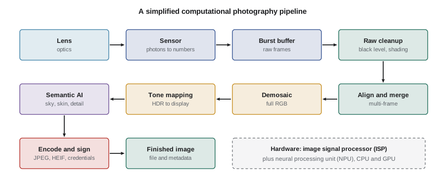
The pipeline from photons to pixels
Every digital camera, phone or not, runs an image processing pipeline. The details are proprietary and change often, but the stages are broadly similar.
- Capture: the sensor converts photons into electrons in each photosite, and an analogue-to-digital converter turns the charge into numbers. Phones typically capture a continuous stream of frames into a ring buffer even before you press the shutter, so the frames used may come from just before the press.
- Raw processing: black level subtraction, correction for defective pixels, lens shading correction and linearization produce a clean raw image in which values are proportional to light.
- Multi-frame processing: several frames are aligned and merged to reduce noise, extend dynamic range or increase resolution.
- Demosaicing: the colour filter array leaves each pixel with only one colour sample; demosaicing estimates the missing two.
- Colour processing: white balance and a colour correction matrix map the sensor's colour response to a standard colour space.
- Tone mapping: the high dynamic range data is compressed into the limited range of a display or file, often with local adjustments.
- Semantic and AI processing: neural networks segment the scene into regions such as sky, skin, hair and foliage and treat each differently, and may denoise, sharpen or upscale.
- Encoding: the image is compressed into JPEG, HEIF or another format, with metadata and, increasingly, a signed provenance record.
Two kinds of hardware share this work. The image signal processor (ISP) is a fixed-function circuit designed to do classic operations very quickly with little power. The neural processing unit (NPU) runs machine learning models. The main processor and graphics processor handle the rest. Much of the progress in phone photography since about 2016 has come from software and these accelerators rather than from optics.
A short history of computational photography
Computational photography grew out of research in computer vision and computer graphics. Paul Debevec and Jitendra Malik's 1997 work on recovering high dynamic range radiance maps from several exposures laid groundwork for HDR photography. Researchers at Stanford, MIT and elsewhere developed light-field cameras, coded apertures and flash/no-flash fusion in the 2000s. The idea of a "camera that computes" moved into consumer products in the 2010s. Google's HDR+ burst pipeline, described in a 2016 paper by Samuel Hasinoff and colleagues, merged several deliberately underexposed frames to reduce noise and preserve highlights. Apple introduced Portrait mode with simulated depth of field in 2016, Google's Night Sight arrived in 2018, and multi-frame super-resolution for zoom followed in 2018 and 2019. Since then, machine learning has spread through every stage, and from about 2022 generative AI added the ability to create or replace image content outright.
Dedicated cameras adopted computation more slowly but now use it too: in-camera HDR, pixel-shift high-resolution modes, focus stacking, live composite modes for night photography, subject-recognition autofocus driven by neural networks and AI-based noise reduction in raw converters. The difference is one of emphasis. A dedicated camera's large sensor and lens collect enough light that computation is optional; a phone depends on it.
Raw, processed and computational raw
A raw file records sensor values with minimal processing, as PHOT-201 explained. On a phone, the meaning of "raw" is complicated. A single-frame raw from a phone sensor is noisy and has limited dynamic range. Several manufacturers therefore offer a computational raw: a file in a raw format, typically Adobe's Digital Negative (DNG), that contains the result of multi-frame merging but has not yet been demosaiced, tone mapped or sharpened, or has been demosaiced but kept linear. Apple ProRAW and Google's raw output from merged bursts are examples. These files give editors the low noise of merging with much of the flexibility of raw.
For photographers this means three choices on a phone: the processed image (JPEG or HEIF), with all of the manufacturer's choices baked in; a computational raw, which keeps merging benefits but leaves tone, colour and sharpening to you; and a single-frame raw from a third-party app, which is the most "honest" sensor record but the noisiest. Understanding the pipeline helps you choose. For documentary work where you must explain what processing occurred, knowing which stages ran is part of professional practice, as lesson 11 discusses.
| Capture type | Multi-frame merging | Tone mapping and sharpening | Typical use |
|---|---|---|---|
| Processed JPEG or HEIF | Yes | Applied by camera | Everyday sharing, fast delivery |
| Computational raw (DNG) | Yes | Mostly left to the editor | Editing with low noise and wide latitude |
| Single-frame raw | No | None | Technical tests, maximum control, forensics |
What computation can and cannot do
It is useful to separate three things computation does. First, it can measure better: combining frames averages away random noise, and that improvement is real information gathered over a longer total time. Second, it can interpret: tone mapping and colour choices decide how measured light looks, and different choices produce different but equally truthful renderings. Third, it can invent: learned models fill in detail that was never captured, such as texture during upscaling, a blurred background in Portrait mode, or new objects in generative fill. Invention can be convincing, but it is not measurement.
These categories overlap. AI denoising, for example, mostly measures and interprets, but at high strength it begins to invent plausible texture. A famous controversy illustrates the line: in 2023 a user photographed a deliberately blurred image of the Moon on a monitor with a phone's high zoom and the phone produced a crisp Moon with crater detail that was not in the source. The manufacturer explained that a scene-optimization model recognized the Moon and enhanced detail. Whatever one thinks of it, the result included learned detail rather than captured detail. Professionals need to know when their tools cross from measurement to invention, because clients, editors, courts and audiences may care.
Signal, noise and the photon budget
Most of computational photography is about noise. Light arrives as discrete photons, and the number arriving at a pixel in a given time varies randomly even under perfectly steady light. This photon shot noise follows Poisson statistics: if a pixel receives on average \( N \) photons, the standard deviation is \( \sqrt{N} \). The signal-to-noise ratio (SNR) from shot noise alone is therefore:
More light means better SNR, but only by the square root. Collecting four times as many photons doubles the SNR. Sensors add further noise, notably read noise from the electronics, which matters most in the darkest tones. A small pixel collects fewer photons than a large one in the same light, so its SNR is lower. Merging frames is a way to collect more photons without a longer single exposure, which would blur with hand or subject motion.
Worked problem
Shot noise in a bright and a dark tone
A pixel collects on average 10,000 photoelectrons in a highlight and 100 in a shadow during one exposure. Ignoring read noise, compare the SNR.
Show solution
- Highlight: \( \sqrt{10\,000} = 100 \), so SNR is 100:1.
- Shadow: \( \sqrt{100} = 10 \), so SNR is 10:1.
- The shadow has 100 times less signal but only 10 times less SNR, yet a 10:1 SNR is visibly noisy.
Answer: SNR is 100 in the highlight and 10 in the shadow; shadows are where noise shows, which is why multi-frame merging and denoising focus there.
Worked problem
How many frames to double the SNR?
A phone merges identical, perfectly aligned frames. How many frames are needed to double the SNR of a single frame, and how many to triple it?
Show solution
- Averaging \( n \) frames multiplies SNR by \( \sqrt{n} \).
- Doubling requires \( \sqrt{n} = 2 \), so \( n = 4 \).
- Tripling requires \( \sqrt{n} = 3 \), so \( n = 9 \).
Answer: Four frames double the SNR and nine triple it; returns diminish, which is why phones rarely merge more than about 15 frames in normal light.
Compute budgets and file sizes
Computation is not free. A phone must finish processing quickly enough that the photographer can take the next picture, and it must not drain the battery or overheat. Engineers therefore work within a compute budget for each photo. Data volumes are large: a 50-megapixel sensor read at 12 bits produces about 75 megabytes of raw data per frame, and a burst of ten frames is 750 megabytes to move and process. Many phones capture at a binned resolution, combining four or more pixels into one, and use full resolution only in good light.
megapixels = 50
bits = 12
frames = 10
bytes_per_frame = megapixels * 1e6 * bits / 8
burst = bytes_per_frame * frames
print(f"one raw frame: {bytes_per_frame / 1e6:.0f} MB")
print(f"burst of {frames}: {burst / 1e6:.0f} MB")
# binning 2x2 reduces pixel count by four
binned = burst / 4
print(f"2x2 binned burst: {binned / 1e6:.0f} MB")
# if the pipeline must finish in 0.5 s, required throughput:
for t in (0.5, 1.0, 2.0):
print(f"finish in {t} s needs {binned / 1e9 / t:.2f} GB/s")one raw frame: 75 MB burst of 10: 750 MB 2x2 binned burst: 188 MB finish in 0.5 s needs 0.38 GB/s finish in 1.0 s needs 0.19 GB/s finish in 2.0 s needs 0.09 GB/s
The output shows why binning and dedicated hardware matter. Even after binning, moving and processing hundreds of megabytes in under a second requires memory bandwidth and specialized circuits. This budget shapes every algorithm in the following lessons: the cleverest method is useless if it takes ten seconds per shot.
Who makes the choices
A computational image embodies thousands of decisions made by engineers, image quality teams and product managers long before you press the shutter. They decide how bright faces should be, how blue skies should look, how much noise is acceptable and how sharp edges should appear. These choices differ between manufacturers and change with software updates, which is why the same scene can look quite different on two phones. Some brands favour a bright, punchy look; others aim for more natural contrast. Some offer "styles" that let users adjust the look before capture, applied within the pipeline rather than as a filter afterward.
For professional photographers the lesson is to treat the phone as an opinionated collaborator. When consistency matters, such as a product catalogue shot partly on a phone, lock what you can (exposure, white balance, style), shoot computational raw where possible, and test how the pipeline treats your typical subjects. When authenticity matters, know what the device did and be ready to explain it.
The structure of this course
The course moves from measurement toward invention. Lessons 2 to 7 cover classic computational photography: the image signal processor, burst capture, HDR and tone mapping, depth and synthetic bokeh, night modes and super-resolution. Lesson 8 covers AI enhancement: denoising, sharpening and upscaling with neural networks. Lessons 9 and 10 cover generative AI: how diffusion and related models work, and how professionals use generative editing ethically and within client, contest and stock rules. Lesson 11 covers authenticity, provenance, content credentials, detection and the law in Canada and the United States. Lesson 12 is a capstone in which you design a computational pipeline and write a provenance and AI-use policy for a photography practice. Several lessons include short Python programs using NumPy with seeded random numbers, so the outputs shown are reproducible and you can experiment by changing parameters.
Common mistakes
MistakeThinking a phone photo is a single exposure
InsteadRecognize that most phone photos are merged from several frames and heavily processed by the pipeline.
MistakeBelieving computation can create real information from nothing
InsteadDistinguish measurement (more photons), interpretation (rendering choices) and invention (learned guesses).
MistakeExpecting a phone raw file to be unprocessed
InsteadCheck whether a raw file is a single-frame raw or a computational raw that already includes merging.
MistakeAssuming noise falls in proportion to the number of frames
InsteadRemember that SNR improves only with the square root of the number of frames.
MistakeIgnoring the manufacturer's rendering choices when consistency matters
InsteadLock settings, shoot computational raw and test the pipeline with your typical subjects.
Summary and key terms
- Computational photography uses algorithms, often including machine learning, to produce images no single exposure could deliver.
- Phones depend on computation because small sensors and thin lenses limit light, depth of field, zoom and dynamic range.
- A typical pipeline runs capture, raw cleanup, multi-frame merging, demosaicing, colour processing, tone mapping, semantic AI processing and encoding.
- Computational raw files keep merging benefits while leaving tone and colour decisions to the editor.
- Operations range from measurement through interpretation to invention, and professionals should know which they are using.
- Shot noise gives an SNR of \( \sqrt{N} \), and averaging \( n \) frames improves SNR by \( \sqrt{n} \).
- Compute, memory and power budgets constrain which algorithms a camera can run.
- Computational photography
- The use of computation, including machine learning, to create images beyond what a single optical exposure can record.
- Image signal processor (ISP)
- A dedicated chip or circuit that performs standard image processing steps quickly and efficiently.
- Neural processing unit (NPU)
- A processor designed to run machine learning models efficiently.
- Computational raw
- A raw-format file containing merged multi-frame data before most rendering decisions.
- Photon shot noise
- Random variation in the number of photons arriving, with standard deviation equal to the square root of the mean.
- Signal-to-noise ratio (SNR)
- The ratio of the mean signal to its standard deviation; higher is cleaner.
- Ring buffer
- Memory that continuously stores the most recent frames so that frames from before the shutter press can be used.
- Binning
- Combining neighbouring pixels into one to reduce noise and data volume at the cost of resolution.
- Semantic segmentation
- Labelling each pixel by the kind of content it shows, such as sky, skin or foliage.
- Compute budget
- The time, energy and memory available to process each photo.
Practice problems
Work each problem on paper first, then reveal the answer to check.
List three physical limits of phone cameras and the computational response to each.
Show answer
Small sensors and noise: burst merging; limited dynamic range: multi-frame HDR; deep depth of field: synthetic bokeh (also limited zoom: super-resolution).
Why does a phone capture frames before the shutter is pressed?
Show answer
So the pipeline can use frames from the moment of the press, reducing shutter lag and supplying extra frames for merging.
A pixel receives 400 photons on average. What is its shot-noise SNR?
Show answer
\( \sqrt{400} = 20 \).
How many perfectly aligned frames are needed to improve SNR by a factor of 5?
Show answer
\( 5^2 = 25 \) frames.
Classify synthetic bokeh as measurement, interpretation or invention, and explain.
Show answer
Largely invention: the blur is simulated from estimated depth, not optically recorded.
What is the difference between a single-frame raw and a computational raw?
Show answer
A single-frame raw is one sensor readout; a computational raw contains merged frames, usually before tone mapping.
Calculate the size of one 12-bit raw frame from a 48-megapixel sensor.
Show answer
\( 48 \times 10^6 \times 12 / 8 = 72 \) MB.
Why might two phones render the same scene differently?
Show answer
Their manufacturers make different tone, colour, noise and sharpening choices in their pipelines.
Name two kinds of hardware that share phone image processing.
Show answer
The image signal processor and the neural processing unit (also the CPU and GPU).
Give one reason a photojournalist should know which pipeline stages ran on an image.
Show answer
To explain processing honestly to editors and audiences and to avoid using invented detail in documentary work.
Lesson quiz · 5 questions
Score 60% or more to complete this lesson.
Create a free account to save your progress, take quizzes and earn a certificate.