
PET-499 · Lesson 8 of 12 · 22 min
Production forecasting and artificial lift
Every later part of the plan runs on the production forecast: the facility sizes, the operating costs, the revenue and therefore the value, the emissions and the reserves that could be booked. Mateo and Hannah share the work. Mateo builds the forecasts of oil, water and gas for each option and each aquifer case; Hannah works out how the wells will be kept producing as the water cut rises. Ethan's instruction is to keep the forecasting method simple enough that the committee can follow it, but to be explicit about every assumption.
A forecasting method for the select stage
At this stage the team cannot run a full simulation for every option and case, and it would not be credible if it did, given the data. Instead it uses a method common in early field planning: estimate the ultimate recovery for each option and case, then shape a production profile that delivers it within the limits of the wells and the facilities. The recovery comes from the reservoir work. The shape comes from three rules.
First, the rate is limited by the capacity of the wells and the facility. The facility limit is a design choice, made later in the light of the forecast; the team starts with a plateau sized to produce the reserves of the waterflood case at a sensible pace. The well limit comes from Lesson 7: about 90 m³/d for a vertical well, held near its practical coning limit, and about 160 m³/d for a horizontal well. Second, once the reservoir can no longer sustain the plateau, the rate declines in proportion to the remaining recoverable oil, so that each year the field produces a fixed fraction of what is left. That gives an exponential decline after the plateau. Third, the facilities are available 95 percent of the time, to allow for maintenance, upsets and well work.
The decline constant k is set at 0.20 per year, a value typical of well-supported carbonate pools of this size, so that after the plateau the field produces a fifth of its remaining reserves each year. For depletion with a weak aquifer, where the reservoir quickly falls into solution-gas drive, a faster value of 0.28 is used. The water cut rises with the fraction of the ultimate recovery produced, steeply at first and then levelling off, towards 85 percent at the end of life in the supported cases and 40 percent in the weak depletion case, where there is little water to produce.
Recovery for each option and case
The ultimate recovery of each option and aquifer case combines the tank results of Lesson 6, the analogue recovery ranges of Lesson 5 and the sector model's estimate of sweep. Mateo presents them as fractions of the P50 oil in place.
| Option | Weak aquifer | History-matched aquifer | Strong aquifer | Main reason for the range |
|---|---|---|---|---|
| A: depletion, verticals | 15% | 25% | 31% | Pressure support depends entirely on the aquifer; weak case falls below the bubble point |
| B: horizontals and waterflood | 34% | 35% | 36% | Injection maintains pressure in every case; limited by sweep with three producers |
| C: phased | 32% | 33% | 34.5% | Injection added after 18 months in the weak and matched cases; not added in the strong case |
Two features of the table are worth noting. The waterflood recovery of about 35 percent is below the most likely value of 38 percent in the Lesson 5 range, because the select-stage design has only three producers; a full pattern of wells would sweep more of the reef but would cost far more. And option C recovers slightly less than option B in every case, because injection, where it is added, starts later and because the third horizontal producer is not drilled; in the strong case it relies on the aquifer, which then behaves almost like a flood.
# Production forecasts for the three development options and three aquifer cases, and the gas-lift requirement.
SI = True      # True: Canadian case (m3/d), False: US case (bbl/d)
N = 1.825e6 if SI else 8.105e6                  # P50 oil in place, m3 or STB
cap = 320.0 if SI else 1600.0                    # facility oil limit per day
qv, qh = (90.0, 160.0) if SI else (450.0, 800.0)  # per-well rate limits: vertical (coning), horizontal
gor = 150.0 if SI else 900.0                     # solution gas-oil ratio, m3/m3 or scf/STB
u = "m3/d" if SI else "bbl/d"
RF = {"A": {"weak": 0.15, "matched": 0.25, "strong": 0.31},   # three verticals, depletion
      "B": {"weak": 0.34, "matched": 0.35, "strong": 0.36},   # three horizontals, two injectors
      "C": {"weak": 0.32, "matched": 0.33, "strong": 0.345}}   # two horizontals and 14-09, injection decision after 18 months

def forecast(opt, aq, years=25):
    """Yearly oil, water cut and per-day rates. Rate = min(capacity, 0.20 of remaining reserves per year)."""
    eur = N * RF[opt][aq]; k = 0.28 if (opt == "A" and aq == "weak") else 0.20
    wmax = 0.40 if (opt == "A" and aq == "weak") else 0.85
    rows, Np = [], 0.0
    for y in range(years):
        if opt == "A": capy = 3 * qv
        elif opt == "B": capy = cap
        else: capy = 2 * qh + qv               # two horizontals and the discovery well; Phase 2 adds injection unless the aquifer is strong
        if opt == "C" and y < 2: eur_y = N * 0.30  # until injection starts, recovery is that of the natural drive
        else: eur_y = eur
        q = min(min(capy, cap) * 365 * 0.95, k * (eur_y - Np))
        Np += q; wc = wmax * (Np / eur) ** 1.5
        rows.append((y + 1, q / 365, wc, Np))
    return rows, eur

for opt, name in (("A", "A: three verticals, depletion"), ("B", "B: horizontals and waterflood"), ("C", "C: phased")):
    rows, eur = forecast(opt, "matched")
    print(f"{name} (history-matched aquifer): EUR {eur / 1e6:.3f} million {'m3' if SI else 'bbl'}")
    print("   " + "  ".join(f"y{y}:{q:,.0f}" for y, q, wc, _ in rows[:8]) + f"  ({u})")
    y50 = next((y for y, q, wc, _ in rows if wc >= 0.5), None)
    print(f"   water cut reaches 50 percent in year {y50}; cumulative after 10 years {rows[9][3] / eur * 100:.0f} percent of EUR")
print("EUR by aquifer case (million " + ("m3" if SI else "bbl") + "):")
for opt in "ABC":
    print(f"   {opt}: " + ", ".join(f"{aq} {N * RF[opt][aq] / 1e6:.3f}" for aq in ("weak", "matched", "strong")) +
          f"; spread {100 * (RF[opt]['strong'] - RF[opt]['weak']) / RF[opt]['matched']:.0f} percent of the matched case")

# Gas lift for a horizontal producer at 50 percent water cut: inject enough gas to reach the target gas-liquid ratio.
qliq = qh                                        # total liquid per well when the cut is 50 percent
glr_form = gor * 0.5                             # formation gas per unit of liquid
glr_target = 180.0 if SI else 1000.0             # total gas-liquid ratio for good lift at this depth (from a lift design chart)
inj = (glr_target - glr_form) * qliq
tot = f"{3 * inj:,.0f} m3/d" if SI else f"{3 * inj / 1e6:.2f} MMscf/d"
print(f"gas lift at 50 percent water cut: formation GLR {glr_form:.0f}, injection {inj:,.0f} " +
("m3/d" if SI else "scf/d") + f" per well, {tot} for three wells")A: three verticals, depletion (history-matched aquifer): EUR 0.456 million m3 y1:250 y2:200 y3:160 y4:128 y5:102 y6:82 y7:66 y8:52 (m3/d) water cut reaches 50 percent in year 6; cumulative after 10 years 89 percent of EUR B: horizontals and waterflood (history-matched aquifer): EUR 0.639 million m3 y1:304 y2:289 y3:231 y4:185 y5:148 y6:118 y7:95 y8:76 (m3/d) water cut reaches 50 percent in year 6; cumulative after 10 years 89 percent of EUR C: phased (history-matched aquifer): EUR 0.602 million m3 y1:300 y2:240 y3:222 y4:178 y5:142 y6:114 y7:91 y8:73 (m3/d) water cut reaches 50 percent in year 6; cumulative after 10 years 89 percent of EUR EUR by aquifer case (million m3): A: weak 0.274, matched 0.456, strong 0.566; spread 64 percent of the matched case B: weak 0.621, matched 0.639, strong 0.657; spread 6 percent of the matched case C: weak 0.584, matched 0.602, strong 0.630; spread 8 percent of the matched case gas lift at 50 percent water cut: formation GLR 75, injection 16,800 m3/d per well, 50,400 m3/d for three wells
With the history-matched aquifer, option A's three verticals start at 250 m³/d and decline from the first year, because the reservoir cannot sustain the wells' combined rate for long without injection. Option B holds the facility plateau of 304 m³/d (320 m³/d at 95 percent uptime) for two years before declining. Option C starts at about the same rate as B, falls a little in its second year until injection is added, and then follows B closely. The ultimate recoveries tell the main story. Option A recovers anywhere from 0.27 to 0.57 million m³ depending on the aquifer, a spread of 64 percent of its matched case; option B recovers 0.62 to 0.66 million m³, a spread of only 6 percent; option C sits just below B, with a spread of 8 percent.
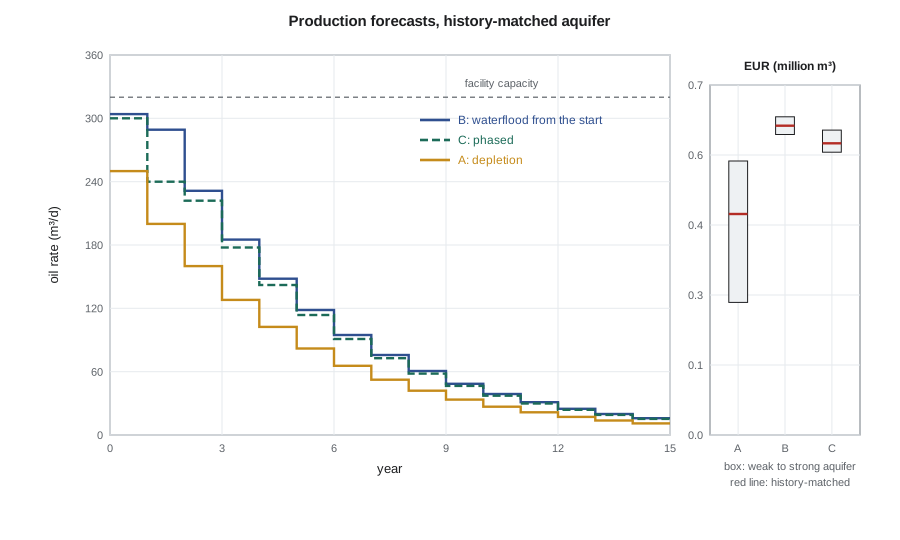
In all three options, about 89 percent of the ultimate recovery is produced in the first ten years, and the water cut reaches 50 percent in about the sixth year. The water production matters as much as the oil for the facility design: by the end of field life the battery will handle four barrels of water for every barrel of oil. In option B and in option C with injection, almost all of that water is reinjected, which closes the loop. In option A the produced water must be disposed of in a disposal well, which the plan must also include.
Gas forecasts
While the reservoir stays above the bubble point, the producing gas-oil ratio is simply the solution gas-oil ratio, so the gas forecast is the oil forecast multiplied by 150 m³/m³. That is one of the practical advantages of pressure maintenance: the gas plant can be contracted for a predictable volume. In option A with a weak aquifer the reservoir falls below the bubble point within the first few years, free gas reaches the wells, and the producing gas-oil ratio would climb to several times the solution value before falling as the gas is depleted. The gas plant contract and the pipeline would have to be sized for that peak, which is another hidden cost of depletion.
Keeping the wells producing: artificial lift
At first the Spruce Ridge wells will flow naturally. The reservoir pressure is close to hydrostatic, the oil is light and gassy, and the column of oil and gas in the tubing is much lighter than the pressure in the reservoir can support. As the water cut rises, the column gets heavier, because water is denser than oil and brings no gas with it. At some point, which Hannah estimates from a tubing performance calculation to be around a water cut of 30 to 40 percent, the wells will stop flowing at the desired rate and need artificial lift.
The choice of lift method is a screening exercise against the well's conditions: depth, rate, deviation, gas-liquid ratio, temperature and the sour fluid. The team considers four methods.
| Method | Suitability at Spruce Ridge | Main concerns |
|---|---|---|
| Rod pumping | Poor | Deep wells and high rates exceed practical rod loads; rod and tubing wear in deviated wells |
| Electrical submersible pump (ESP) | Possible | High gas-liquid ratio needs gas handling at the pump; replacement needs a workover rig; sour-service materials |
| Gas lift | Good | Needs a gas supply and compression; injection gas is sour, so compressors and lines are sour-rated |
| Plunger lift | Unsuitable | Intended for low-rate gas wells unloading liquids |
Gas lift wins the screening. It injects gas into the tubing through valves set at depth, lightening the column so that the reservoir pressure can lift it. It has few moving parts downhole, tolerates the deviated and horizontal wells, handles high gas-liquid ratios, and can be adjusted from the surface as conditions change. The gas is available: the field produces it, and the battery can compress part of the solution gas and send it back down the wells in a closed loop, so the lift gas is not consumed. The main cost is the compressor. An ESP would be more energy-efficient at high water cuts and is kept as an option for later life, if a well's rate justifies the workover costs.
The last part of the code estimates how much gas the wells will need. A common design target is a total gas-liquid ratio in the tubing that gives a near-minimum flowing pressure gradient at the well's depth and rate, read from gas-lift design charts. The injection rate is then the difference between that target and the formation gas, times the liquid rate.
At 50 percent water cut and 160 m³/d of total liquid per well, the formation gas-liquid ratio is 75 m³/m³ and the target is about 180 m³/m³, so each well needs about 16,800 m³/d of lift gas and the three producers about 50,400 m³/d. That is roughly the same as the solution gas the field produces at plateau, so the compressor is a significant piece of equipment, sized in Lesson 9.
Worked problem
When will gas lift be needed?
In option B, the water cut is modelled as 0.85 × (Np/EUR)^1.5. Hannah's tubing calculation shows the horizontal wells stop flowing at the design rate at a 35 percent water cut. What fraction of the ultimate recovery has then been produced, and roughly when?
Show solution
- Solve 0.35 = 0.85 × x^1.5 for x = Np/EUR: x^1.5 = 0.412, so x = 0.412^(2/3) = 0.55.
- From the option B profile, cumulative production reaches 55 percent of EUR during the fourth year.
- Gas lift should therefore be installed in the wells at completion, with dummy valves, and the compressor brought into service in year 3 or 4.
Answer: Gas lift will be needed from about the fourth year. Installing the mandrels at completion avoids a workover later, which is expensive in a sour well; the compressor can be added when it is needed, but the battery layout must leave room for it.
Forecast uncertainty
The forecasts for the history-matched aquifer are the base case, but the team presents every option across all three aquifer cases and, in Lesson 10, at the P90 oil in place. The committee should see that the depletion option's outcome depends heavily on something the company does not yet know, while the waterflood options are robust to it. That robustness is the main argument for injection; its cost is the subject of the economics.
Common mistakes
MistakeBuilding detailed profiles from an unconstrained simulation at the select stage.
InsteadUse recovery factors with explicit, documented profile rules; build the simulation model when the data can support it.
MistakeAssuming a constant gas-oil ratio below the bubble point.
InsteadAbove the bubble point the ratio is constant; below it the producing ratio climbs, which affects gas facilities.
MistakeChoosing a lift method by habit.
InsteadScreen methods against depth, rate, deviation, gas-liquid ratio, temperature and sour service.
MistakeWaiting to install gas-lift mandrels until the wells stop flowing.
InsteadInstall mandrels at completion to avoid expensive sour-well workovers later.
Summary and key terms
- Select-stage forecasts combine ultimate recovery estimates with simple, explicit profile rules: capacity limits, decline in proportion to remaining reserves, and uptime.
- Depletion recovery at Spruce Ridge depends strongly on the aquifer; waterflood recovery hardly at all.
- About 89 percent of recovery comes in the first ten years; the water cut reaches 50 percent in about year six.
- Above the bubble point, the gas forecast is the oil forecast times the solution gas-oil ratio.
- Gas lift suits deep, deviated, gassy, sour wells; it needs compression and is installed with mandrels at completion.
- Lift-gas demand at Spruce Ridge is comparable to the field's own gas production.
- Plateau
- The period in which production is held at the facility or well capacity.
- Uptime
- The fraction of time facilities and wells are producing.
- Water cut
- The fraction of produced liquid that is water.
- Gas lift
- Artificial lift by injecting gas into the tubing to lighten the fluid column.
- Gas-liquid ratio
- The volume of gas produced or present per unit volume of liquid.
- Electrical submersible pump (ESP)
- A multistage centrifugal pump driven by a downhole electric motor.
Practice problems
Work each problem on paper first, then reveal the answer to check.
Why does a rising water cut eventually stop a well from flowing?
Show answer
Water is denser than oil and carries no gas, so the column in the tubing becomes heavier than the reservoir can lift.
In the profile model, what produces an exponential decline after the plateau?
Show answer
Producing a fixed fraction of the remaining recoverable oil each year.
Why is rod pumping a poor fit for the Spruce Ridge producers?
Show answer
The wells are deep, high-rate and deviated, which exceed practical rod loads and cause wear.
Why is the gas forecast simple while the reservoir stays above the bubble point?
Show answer
The producing gas-oil ratio equals the constant solution gas-oil ratio.
Lesson quiz · 5 questions
Score 60% or more to complete this lesson.
Create a free account to save your progress, take quizzes and earn a certificate.