
PET-420 · Lesson 7 of 12 · 20 min
Building a reservoir model: grids, upscaling and properties
The geologist's static model of the Cardium A pool contains about four million cells, each roughly 25 m (82 ft) square and less than 0.5 m (1.6 ft) thick, with porosity, permeability, facies and water saturation populated from logs, core and a geostatistical model. Lena's simulation model will have about 150,000 active cells. Turning the first into the second is the subject of this lesson: designing the simulation grid, upscaling the fine-scale properties onto it and assigning the rock and fluid data that the flow equations need. 'This is where the geology either survives or gets averaged away,' Lena tells Ethan. 'Our main uncertainty is a thin layer that carries most of the flow. If the grid smears it into its neighbours, no amount of history matching will put it back.'
Designing the grid
Grid design starts from the questions the model must answer and the features that control flow. Areally, the blocks must be small enough that there are several between each injector and producer, so the waterfront can be resolved; a common rule is at least five to ten blocks between wells. Vertically, the layering must preserve barriers, baffles and high-permeability streaks. The grid should follow the main faults and the structure, which usually means a corner-point grid whose layers follow the stratigraphy and whose columns are aligned with the main faults. Where possible, the grid axes should also follow the main flow directions between injectors and producers, to reduce the grid orientation effects mentioned in Lesson 3.
Lena's grid uses 50 m (164 ft) blocks areally, which places about eight blocks between the pilot injector and each producer at the usual well spacing of the pool. Vertically, it has twelve layers through the reservoir interval, chosen by the geologist and Ethan so that the thin high-permeability layer and the two shale breaks each have their own simulation layer. A coarser area outside the pilot extends the model to the edges of the pool so that pressure communication with the rest of the reservoir and the aquifer is represented.
Two refinements are common. Local grid refinement (LGR) subdivides blocks around wells, fronts or fractures into finer cells while leaving the rest of the grid coarse. It is used around horizontal wells, around hydraulic fractures and where coning of water or gas is important. Grid coarsening does the opposite in regions where little happens, such as the aquifer. Both reduce the number of cells without losing resolution where it matters, but the interfaces between fine and coarse regions require careful transmissibility calculation.
Why upscaling is needed
A fine-scale static model contains detail that the simulation grid cannot hold. Each simulation block contains many fine cells, and a single value of porosity, permeability and other properties must represent them all. For additive properties such as pore volume, the answer is simple: sum the fine-cell pore volumes, or equivalently use a bulk-volume-weighted average porosity. For saturation, use a pore-volume weighting. Permeability is harder, because it is not additive. The effective permeability of a block depends on how the fine-scale values are arranged and on the direction of flow.
Two arrangements have exact answers. When layers lie parallel to the flow, each carries flow in proportion to its permeability-thickness, and the effective permeability is the thickness-weighted arithmetic average. When layers lie across the flow, they act as resistances in series, and the effective permeability is the thickness-weighted harmonic average:
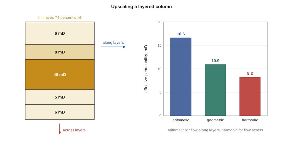
The arithmetic average is always the largest and the harmonic the smallest; the true effective value of any arrangement lies between them. For a statistically random field with no spatial correlation in two dimensions, the effective permeability is close to the geometric average, which lies between the two bounds. The code below applies the three averages to the five fine layers of one simulation layer in the pilot, which contains a thin high-permeability streak, and to a random field.
# Upscaling layer permeabilities: arithmetic, harmonic and geometric averages
import math, random
SI = True
# fine layers of the pool: thickness (m) and permeability (mD); one thin high-permeability layer
layers = [(1.5, 6.0), (1.0, 8.0), (2.0, 40.0), (1.0, 5.0), (1.0, 6.0)]
H = sum(t for t, _ in layers)
k_arith = sum(t * k for t, k in layers) / H          # flow along the layers (horizontal)
k_harm = H / sum(t / k for t, k in layers)          # flow across the layers (vertical)
k_geo = math.exp(sum(t * math.log(k) for t, k in layers) / H)
share = layers[2][0] * layers[2][1] / sum(t * k for t, k in layers)
hu, hf = ("m", 1) if SI else ("ft", 3.28084)
print(f"total thickness {H * hf:.1f} {hu}")
print(f"arithmetic (kh / h), horizontal: {k_arith:5.1f} mD")
print(f"harmonic, vertical:               {k_harm:5.1f} mD")
print(f"geometric:                        {k_geo:5.1f} mD")
print(f"thin layer carries {100 * share:.0f} percent of the flow capacity kh")
# random (uncorrelated) field: geometric mean is the usual 2D estimate
random.seed(7)
field = [math.exp(random.gauss(math.log(15), 0.8)) for _ in range(4000)]
print(f"random field: arithmetic {sum(field) / len(field):.1f}, geometric "
f"{math.exp(sum(map(math.log, field)) / len(field)):.1f}, harmonic {len(field) / sum(1 / x for x in field):.1f} mD")total thickness 6.5 m arithmetic (kh / h), horizontal: 16.6 mD harmonic, vertical: 8.2 mD geometric: 10.9 mD thin layer carries 74 percent of the flow capacity kh random field: arithmetic 20.6, geometric 15.0, harmonic 10.8 mD
The streak is only 2 m (6.6 ft) of 6.5 m (21.3 ft) but carries about three quarters of the flow capacity, consistent with the injection profiles from the pilot. The horizontal effective permeability is about twice the vertical. If the five layers are combined into one simulation layer, the model will move water through the full thickness at the averaged rate and will predict breakthrough later and a more even sweep than reality. That is why Lena insists the streak keep its own layer. The random field shows the other key result: the three averages differ widely even for an uncorrelated field, so the choice of method matters.
In real three-dimensional heterogeneity, no simple average is exact. Flow-based upscaling solves a small single-phase flow problem on the fine cells of each coarse block, or on a slightly larger region around it, with pressure applied on two opposite faces, and computes the effective permeability from the resulting flow. This is done separately for each direction. Transmissibility upscaling goes one step further and computes the coarse face transmissibilities directly, which handles barriers that lie between coarse blocks more accurately. Most geomodelling packages offer these methods.
Upscaling multiphase properties
Upscaling single-phase permeability does not preserve multiphase behaviour. A coarse block containing a thin, fast streak and thick, slow layers will see water arrive along the streak long before the rest of the block is swept. Using the fine-scale relative permeability curves in that block, with the averaged permeability, makes the block flood too evenly. One remedy is pseudo-relative permeabilities, curves derived from fine-scale two-phase simulations so that the coarse model reproduces the fine-scale fluxes. The classic methods of Kyte and Berry and of Jacks and others date from the 1970s. Pseudo-curves can work well but are specific to the flow conditions under which they were derived, and many engineers prefer to keep enough vertical resolution that the original curves remain valid.
Numerical dispersion, discussed in Lesson 9, also depends on the grid. Coarse blocks smear fronts and advance them faster. Upscaling and numerical dispersion therefore interact, and both are reasons to compare a coarse model with a fine cross-section before trusting it.
Rock and fluid properties
Each block also needs rock-type-dependent properties: relative permeability and capillary pressure curves, rock compressibility and, for some studies, a permeability-porosity relationship. Special core analysis provides a handful of measured curves, which are grouped by rock type or facies and normalized by their endpoint saturations so that the model can scale them to the irreducible water and residual oil saturation of each block. This endpoint scaling allows one set of curve shapes to serve blocks with different saturation endpoints.
The fluid description comes from the PVT report: black-oil tables of B_o, R_s and μ_o versus pressure, gas properties, water properties and surface densities. For a pool with a single fluid, one table suffices. Large pools may have several PVT regions or a bubble point that varies with depth. Ethan builds the tables from the same laboratory data used in earlier material balance work, and checks that the simulated oil in place at initial conditions reproduces the volumetric estimate.
Special reservoir types
Naturally fractured reservoirs, common in carbonates and in some tight sandstones, have two pore systems: a fracture network with high permeability and low pore volume, and a matrix with most of the pore volume and low permeability. Dual-porosity models represent each block as a fracture cell and a matrix cell, with flow between blocks only in the fractures and an exchange term, controlled by a shape factor, between matrix and fracture within each block. Dual-permeability models also allow matrix-to-matrix flow between blocks. These models suit reservoirs in which the matrix is too tight to flow over interwell distances but feeds the fractures locally.
Unconventional reservoirs such as the Bakken and the Montney are produced through multistage hydraulically fractured horizontal wells. Simulation models of these wells usually represent each fracture explicitly with a thin, high-permeability column of cells refined logarithmically toward the fracture face, or with a zone of enhanced permeability around the well called the stimulated reservoir volume. Because the matrix permeability is measured in microdarcies or nanodarcies, the pressure transient from each fracture moves slowly, and the cell sizes near the fractures must be very small to capture it. Embedded discrete fracture models are an alternative that represents fractures as separate elements connected to the cells they cross.
| Model feature | Purpose | Typical setting in the pilot model |
|---|---|---|
| Areal block size | Resolve fronts between wells | 50 m (164 ft), about eight blocks between wells |
| Vertical layering | Preserve barriers and streaks | Twelve layers, thief layer and shales kept separate |
| Local grid refinement | Resolve near-well flow | Not needed for vertical pilot wells |
| Saturation function regions | Assign curves by rock type | Three rock types from core and logs |
| PVT regions | Assign fluid tables | One region for the pool |
| Aquifer | Represent pressure support | Analytical aquifer connected to the lower edge |
Worked problem
Upscaling a five-layer column
A simulation layer contains five fine layers with thicknesses 1.5, 1.0, 2.0, 1.0 and 1.0 m (4.9, 3.3, 6.6, 3.3 and 3.3 ft) and permeabilities 6, 8, 40, 5 and 6 mD. Find the horizontal and vertical effective permeabilities and the share of kh in the third layer.
Show solution
- The total thickness is 6.5 m (21.3 ft). Using metres for the weights, Σ k_j h_j = 9 + 8 + 80 + 5 + 6 = 108 mD·m, so k_arith = 108 / 6.5 = 16.6 mD.
- Σ h_j / k_j = 0.25 + 0.125 + 0.05 + 0.20 + 0.167 = 0.792 m/mD, so k_harm = 6.5 / 0.792 = 8.2 mD.
- The third layer has kh = 80 of 108 mD·m, or 74 percent.
Answer: The horizontal permeability is 16.6 mD, the vertical is 8.2 mD and the thin layer carries 74 percent of the flow capacity, as in the code output. The thickness unit cancels, so the result is the same in feet.
Checking the upscaled model
Every upscaled model should be checked against the fine-scale model it came from. The simplest check is volumetric: pore volume and oil in place should agree within a fraction of a percent, region by region. A flow check goes further. Ethan extracts a cross-section of the fine geological model through the pilot injector and two producers, about 20,000 fine cells, and runs the same waterflood on it and on the corresponding slice of the coarse simulation grid. The two give breakthrough times within about a month and water cut curves that differ by a few percent, which confirms that keeping the thief layer separate was enough. When Lena once tried the same comparison with the thief layer merged into its neighbours, the coarse model broke through more than a year late, which is exactly the error the history match would otherwise have had to absorb with unjustified changes elsewhere in the model.
Common mistakes
MistakeUsing the arithmetic average for vertical permeability.
InsteadFlow across layers sees the harmonic average, dominated by the tightest layer.
MistakeCombining a thin high-permeability streak with its neighbours.
InsteadKeep layers that control flow separate, or derive pseudo-relative permeabilities that honour them.
MistakeUpscaling porosity with a simple unweighted average.
InsteadWeight porosity by bulk volume and saturation by pore volume so oil in place is preserved.
MistakeMaking the grid so coarse that wells are one block apart.
InsteadKeep several blocks between injectors and producers so fronts can be resolved.
Summary and key terms
- Grid design follows the questions, the structure, the faults and the features that control flow.
- Local grid refinement adds resolution near wells and fractures without refining the whole model.
- Pore volume and saturations upscale by volume-weighted averages; permeability depends on arrangement and direction.
- The arithmetic and harmonic averages bound the effective permeability; flow-based upscaling handles real heterogeneity.
- Thin high-permeability layers can carry most of the flow and must be preserved in the grid.
- Dual-porosity, refined fracture and stimulated reservoir volume models represent fractured and unconventional reservoirs.
- Upscaling
- Assigning coarse-block properties that reproduce the behaviour of the fine-scale model.
- Flow-based upscaling
- Computing effective permeability from a fine-scale flow simulation over each coarse block.
- Local grid refinement
- Subdividing selected blocks into finer cells while keeping the surrounding grid coarse.
- Pseudo-relative permeability
- A relative permeability curve derived so that a coarse model reproduces fine-scale two-phase flow.
- Endpoint scaling
- Adjusting normalized saturation functions to the endpoint saturations of each block.
- Dual-porosity model
- A model with fracture and matrix cells in each block, linked by a transfer function.
- Stimulated reservoir volume
- The region around a fractured well represented with enhanced permeability.
Practice problems
Work each problem on paper first, then reveal the answer to check.
Why does the arithmetic average apply to flow along layers?
Show answer
Layers in parallel each carry flow in proportion to kh, so capacities add.
What does flow-based upscaling compute?
Show answer
Effective permeability from a small fine-scale flow simulation across each coarse block.
When is a dual-porosity model appropriate?
Show answer
When a fracture network carries flow and a low-permeability matrix holds most of the pore volume.
Why might a coarse model predict breakthrough too late?
Show answer
Averaging a thin fast layer into its neighbours slows the simulated front along that layer.
Lesson quiz · 5 questions
Score 60% or more to complete this lesson.
Create a free account to save your progress, take quizzes and earn a certificate.