
PET-420 · Lesson 10 of 12 · 20 min
History matching
With the model built and initialized, Ethan runs it through the pool's history: fourteen years of primary production and eighteen months of pilot injection, with each producer controlled by its measured liquid rate. The first run is disappointing. The simulated pool pressure falls too fast, the first pilot producer sees water five months late and two of the other producers water out in the model before they have in reality. 'Good,' says Lena. 'Now we know what the model has to learn. History matching is not about making the curves line up. It is about finding out which parts of our description of the reservoir are wrong, and fixing those.'
What is matched
A history match compares the model's predictions with field observations over the period for which both exist. The observations come in a hierarchy. At the top are pool-wide quantities: average pressure from shut-in surveys and the total production of oil, water and gas. Below them are well-level data: each well's water cut, gas-oil ratio and flowing or static pressure. Below those are local measurements that test the vertical description: injection and production profiles from logs, pressure tests and repeat formation tests in new wells that show pressure by layer, tracer arrival times and, in some fields, saturation logs or time-lapse seismic that show where water has gone.
Matching generally proceeds from the top down. The pool pressure is matched first, by adjusting quantities that control the overall energy of the system: pore volume, aquifer size and strength, compressibility and the connection to neighbouring areas. Once the energy balance is right, the fluid movement is matched: breakthrough times, water cut development and gas-oil ratio, by adjusting the properties that control where fluids go, such as layer permeabilities, vertical permeability, fault transmissibilities and relative permeability. Matching the details before the totals usually wastes effort, because changing the pressure match later changes everything else.
The objective function
To judge a match objectively, the misfit between simulated and observed values is summarized in an objective function. The most common is a weighted sum of squared differences:
Here m is the vector of uncertain model parameters, d are the data, σ_i is the measurement uncertainty of each observation and w_i is a weight that expresses how much the engineer trusts or cares about each data type. Dividing by the measurement variance has an important consequence: the match is good when misfits are about the size of the measurement errors, not when they are zero. A model that matches noisy data perfectly has probably been tuned to the noise and will forecast badly.
The weights are a matter of judgement. Pressure surveys from permanent gauges are precise; allocated well rates in a pool with shared test separators are not. Water cuts from monthly tests may scatter by several percent. Lena assigns weights that reflect both the data quality and the purpose of the model: the waterflood forecast depends most on breakthrough and water cut development, so those get a high weight once the pressure is matched.
A pressure match
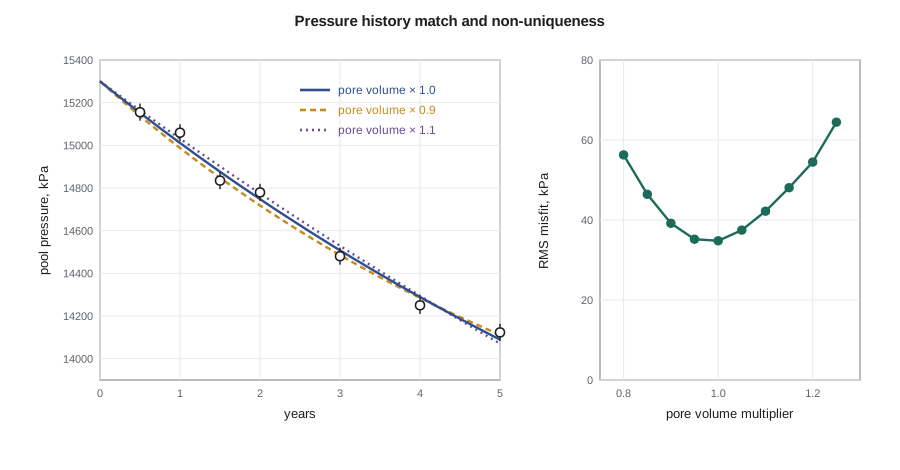
The first step of Ethan's match is the pool pressure. The code below reduces it to its simplest form. The pool is a tank with an analytical Schilthuis aquifer, whose influx is proportional to the pressure drop from the initial pressure. Seven pressure surveys with gauge and averaging errors are available. A golden-section search finds the aquifer constant that minimizes the misfit. The code then repeats the search for several values of the pore volume, to see whether a different combination of oil in place and aquifer strength fits just as well.
# History matching a pool tank model: tune the aquifer constant to fit measured pressures
import random
SI = True
N, Boi, ce, pi = 5.11e6, 1.294, 1.4e-5, 15300.0     # m3, rm3/m3, 1/kPa (effective, includes rock and water), kPa
q_oil, Bo = 60.0, 1.296                             # m3/d oil, rm3/m3
def run(kaq, months=60, pv_mult=1.0):
    p = pi; out = []
    for m in range(months):
        for _ in range(30):                          # daily steps
            influx = kaq * (pi - p)                  # Schilthuis steady-state aquifer, rm3/d
            p -= (q_oil * Bo - influx) / (N * pv_mult * Boi * ce)
        out.append(p)
    return out
random.seed(3)
truth = run(0.020)
obs = {m: truth[m] + random.gauss(0, 40) for m in (5, 11, 17, 23, 35, 47, 59)}   # gauge surveys
def misfit(kaq, pv_mult=1.0):
    sim = run(kaq, pv_mult=pv_mult)
    return sum((sim[m] - v) ** 2 for m, v in obs.items()) / len(obs)
a, b = 0.0, 0.1; g = 0.6180339887                    # golden-section search on the aquifer constant
for _ in range(40):
    c, d = b - g * (b - a), a + g * (b - a)
    if misfit(c) < misfit(d): b = d
    else: a = c
k_best = (a + b) / 2
f, u = (1, "kPa") if SI else (0.145038, "psi")
ka, au = (1, "rm3/d per kPa") if SI else (6.28981 / 0.145038, "rb/d per psi")
print(f"best aquifer constant {k_best * ka:.4f} {au}; RMS misfit {misfit(k_best) ** 0.5 * f:.0f} {u}")
print(f"final pressure: simulated {run(k_best)[-1] * f:.0f}, last survey {obs[59] * f:.0f}")
# non-uniqueness: a bigger pool with a weaker aquifer fits almost as well
for pvm in (0.8, 0.9, 1.0, 1.1, 1.25):
    best = min((misfit(kk / 2000, pvm), kk / 2000) for kk in range(0, 201))
print(f"pore volume x{pvm:4.2f}: best aquifer {best[1] * ka:.4f}, RMS misfit {best[0] ** 0.5 * f:4.0f} {u}")best aquifer constant 0.0238 rm3/d per kPa; RMS misfit 35 kPa final pressure: simulated 14090, last survey 14123 pore volume x0.80: best aquifer 0.0440, RMS misfit 56 kPa pore volume x0.90: best aquifer 0.0340, RMS misfit 39 kPa pore volume x1.00: best aquifer 0.0240, RMS misfit 35 kPa pore volume x1.10: best aquifer 0.0130, RMS misfit 42 kPa pore volume x1.25: best aquifer 0.0000, RMS misfit 64 kPa
The best match has a root-mean-square misfit of about 35 kPa (5 psi), close to the scatter of the surveys themselves, and the simulated final pressure is close to the last survey. That would be a satisfactory match by most standards. The second part of the output is more important. A pore volume ten percent larger with a weaker aquifer, or ten percent smaller with a stronger one, fits nearly as well. The pressure history alone cannot separate oil in place from aquifer support, a classic example of non-uniqueness. Only more data, such as the volumetric estimate, the material balance plot and the aquifer's response to the waterflood, can narrow the range.
Matching fluid movement
With pressure matched, Ethan turns to the water. The early breakthrough at the first pilot producer and the injection profile log both point to the thin high-permeability layer. Increasing that layer's permeability between the injector and the first producer brings breakthrough forward, but it also brings water to the second producer too early. The geologist suggests a channel orientation that would connect the injector to the first producer more strongly than to the others. Ethan represents it with a permeability multiplier in a band of blocks along the channel, consistent with the facies map, and the match at all four producers improves together.
This is the essence of good history matching: changes should be geologically plausible, should be applied over regions that make physical sense and should improve the match in several places at once. A local permeability multiplier around one well that fixes that well and nothing else is a warning sign. So is a parameter pushed to an extreme value, such as a vertical-to-horizontal permeability ratio of 10⁻⁵ in rock where core shows 0.1. Lena keeps a log of every change, its justification and its effect on the objective function, so that anyone reviewing the model later can see what was done and why.
| Parameter | Affects mainly | Typical range of adjustment | Evidence that constrains it |
|---|---|---|---|
| Pore volume | Pressure level, oil in place | A few percent | Volumetrics, material balance |
| Aquifer strength and size | Pressure decline, water influx | Wide | Pressure history, edge well water |
| Layer permeability | Breakthrough, water cut | Factor of two or three | Core, well tests, profiles |
| Vertical permeability | Crossflow, coning, gravity effects | Order of magnitude | Core, shale continuity |
| Fault transmissibility | Compartment pressures | Zero to one | Pressure differences across faults |
| Relative permeability | Water cut shape, recovery | Endpoints and exponents | Special core analysis |
Assisted history matching
Manual matching relies on the engineer's understanding and works well for a few parameters. For many parameters, or to explore non-uniqueness systematically, assisted history matching methods use the computer to search the parameter space. Experimental design and proxy models run a planned set of cases, fit a response surface to the objective function and use it to find good regions cheaply. Evolutionary and other global optimization methods search directly with many runs.
Ensemble methods have become widely used. The ensemble Kalman filter and its smoother variants, such as ensemble smoother with multiple data assimilation (ES-MDA), start from an ensemble of perhaps 100 models drawn from the prior uncertainty in the geology and properties. They run all members through the history and then update every member's parameters together, using the correlations between parameters and simulated data across the ensemble. The result is not one matched model but an ensemble of matched models that represents the remaining uncertainty, ready for the probabilistic forecasts of Lesson 11. These methods can adjust thousands of parameters, including permeability in every block, but they need care: small ensembles can collapse to too little spread, and updates that ignore the geological model can produce unrealistic property fields.
Whatever the method, the engineer must decide when the match is good enough. A common criterion is that misfits are comparable to measurement errors and show no systematic trend, such as a simulated pressure that is too high early and too low late. Another is that further improvement would require changes that the geology does not support. The match is a means to an end: a model that forecasts the decisions it was built for with an honest range of uncertainty.
Worked problem
Weighing a pressure misfit
Seven pressure surveys have a combined gauge and averaging uncertainty of ±40 kPa (±6 psi) each (one standard deviation). Two candidate models give RMS misfits of 35 kPa (5 psi) and 55 kPa (8 psi). Compute the normalized objective function for each and decide whether either is acceptable.
Show solution
- The normalized objective is O = Σ (misfit_i / σ)² = n × (RMS / σ)², with n = 7.
- For the first model, O = 7 × (35 / 40)² ((5 / 6)²) ≈ 5.4 (4.9). For the second, O = 7 × (55 / 40)² ((8 / 6)²) ≈ 13.2 (12.4).
- For data with independent normal errors, a good match has O close to the number of observations, here about 7.
Answer: The first model matches to within the measurement uncertainty and is acceptable. The second has misfits larger than the measurement errors and should be checked for a systematic problem before it is accepted.
Testing the match with a blind period
One of the best tests of a history match is to hold back part of the data. Ethan matches the model to the history up to twelve months after the start of injection and then runs it forward for the remaining six months without further changes, comparing the prediction with what actually happened. The matched model predicts the water cut at the first producer within a few percent and the onset of water at the second producer within about a month. The third producer, which the model predicts will see water in month seventeen, has not yet watered out at month eighteen. That small miss suggests the channel connection to that well is slightly too strong in the model, and it is one of the parameters that the ensemble carries with a wide range.
A blind test is not proof that the model will forecast well over twenty years, but it is far better evidence than a match alone. It also guards against a common temptation: tuning the model to every new data point as it arrives. If a model needs adjustment every month to stay matched, it is describing the data rather than the reservoir. Lena tells Ethan to judge a model by how little it has to change when new data arrive, not by how closely it fits the old data.
Common mistakes
MistakeMatching to zero misfit.
InsteadMatch to within the measurement uncertainty; a perfect match to noisy data overfits.
MistakeFixing each well with its own local multiplier.
InsteadPrefer geologically plausible regional changes that improve several wells at once.
MistakeMatching water cut before matching pressure.
InsteadMatch the energy balance first; pressure changes alter the fluid movement afterward.
MistakeReporting a single matched model as the answer.
InsteadSeveral models fit the data; carry an ensemble or a range of matches into the forecast.
Summary and key terms
- History matching adjusts uncertain model parameters until simulated pressures, rates and water cuts agree with observations.
- Matching proceeds from pool-wide pressure to well-level fluid movement to local layer-by-layer data.
- An objective function sums squared misfits weighted by measurement uncertainty and engineering judgement.
- A good match has misfits comparable to measurement errors, not zero.
- Matches are non-unique: different combinations of parameters can reproduce the same history.
- Assisted and ensemble methods search many parameters and return a set of matched models for forecasting.
- History match
- A model whose simulated performance agrees acceptably with observed field data.
- Objective function
- A single number summarizing the weighted misfit between simulated and observed data.
- Schilthuis aquifer
- An analytical aquifer whose influx rate is proportional to the pressure drop.
- Non-uniqueness
- The existence of several parameter sets that match the history equally well.
- Proxy model
- A fast approximation, such as a response surface, to the simulator output.
- Ensemble Kalman filter
- A method that updates an ensemble of models using correlations between parameters and simulated data.
- ES-MDA
- Ensemble smoother with multiple data assimilation, an iterative ensemble history matching method.
Practice problems
Work each problem on paper first, then reveal the answer to check.
Why is pressure matched before water cut?
Show answer
Pressure reflects the energy balance, and changes to it alter fluid movement afterward.
What does dividing misfits by measurement variance achieve?
Show answer
It makes the match target misfits comparable to data errors rather than zero.
Why is a local multiplier around one well suspicious?
Show answer
It fixes one well without a geological reason and often does not improve the others.
What does an ensemble method deliver at the end of a match?
Show answer
A set of matched models that represents the remaining uncertainty.
Lesson quiz · 5 questions
Score 60% or more to complete this lesson.
Create a free account to save your progress, take quizzes and earn a certificate.