
PET-420 · Lesson 1 of 12 · 22 min
Why simulate: the simulation workflow
Ethan Cardinal's next rotation at Prairie Crest Energy Ltd. brings him back to the reservoir engineering group in Calgary, and back to Lena Haugen, the senior reservoir engineer who mentored him through his first rotation. Two years ago Ethan helped Lena prepare the recommendation that started the Cardium A waterflood pilot: one injector, well 02-22, surrounded by four producers in the down-dip part of the Cardium A pool. The pilot has now been injecting for eighteen months. Water has reached one producer, the other three have responded with higher rates, and management wants to know whether to expand the flood to the whole pool. 'The material balance and the Buckley-Leverett estimate got us this far,' Lena says. 'They cannot tell us which wells to convert, where the water will go through the thief layer or what the pool will produce if we drill a second row of injectors. For that we need a simulation model, and you are going to help me build it and history match it.'
This course is about reservoir simulation: the numerical solution of the equations that describe flow of oil, gas and water through porous rock. A simulator divides the reservoir into many small blocks, writes a mass balance for each fluid in each block, connects neighbouring blocks with Darcy's law and steps the whole system forward in time. The result is a prediction of pressures, saturations and well rates that honours the geology, the fluid properties and the wells in far more detail than a tank model can. This first lesson explains why engineers simulate, what a simulator actually does, how a simulation study is organized and where the method fits among the other tools of reservoir engineering.
From tanks to grids
The material balance treats the whole pool as one tank with one pressure. That is a powerful idea: given production and pressure data, it estimates the oil in place and the drive mechanisms with almost no knowledge of the geology. Its limits are just as clear. A tank has no geometry, so it cannot say where water goes, which well will water out first or how a new well placed in the north of the pool will perform compared with one in the south. Decline curves and analytical waterflood methods add some of this information, but each rests on idealizations such as a single layer, uniform properties or a fixed pattern.
A simulator removes most of those restrictions by dividing the pool into blocks. Each block has its own porosity, permeability, thickness, depth, saturations and pressure. Each block obeys its own material balance, so a simulation model is really thousands or millions of small material balances that exchange fluid with their neighbours. If one block is drained by a well, its pressure falls, fluid flows in from the blocks around it and their pressures fall in turn. If water is injected into a high-permeability layer, it moves rapidly along that layer and reaches the producer sooner than water in the tighter layers above and below. The engineer sees not only how much the pool produces but where and when.
Even a tiny grid shows why this matters. The code below computes the oil in place of a small area as the sum over nine blocks and as a single tank. If the tank's averages are weighted correctly by thickness and pore volume, the two answers agree; if simple arithmetic averages are used, the tank is wrong by a few percent. In a real model the effect is much larger, because the same averaging error enters every flow calculation, not just the volume.
# Why a grid matters: oil in place from a 3 x 3 grid versus one averaged "tank"
SI = True
# each cell: area, net pay, porosity, water saturation
h_m = [4.0, 5.5, 6.0, 6.5, 8.0, 7.5, 6.0, 7.0, 8.0]
phi = [0.11, 0.13, 0.14, 0.14, 0.16, 0.15, 0.13, 0.15, 0.16]
sw = [0.38, 0.32, 0.31, 0.30, 0.27, 0.28, 0.31, 0.29, 0.26]
if SI:
    area, h, Bo, cf, unit = 128 * 1e4, h_m, 1.29, 1e-6, "million m3"   # m2 per cell, m
else:
    area, h, Bo, cf, unit = 52 * 43560, [4.5 * x for x in h_m], 1.29, 1 / 5.6146 * 1e-6, "MMSTB"  # ft2, ft
cells = list(zip(h, phi, sw))
ooip_cells = sum(area * hh * p * (1 - s) / Bo for hh, p, s in cells)
A = 9 * area
h_avg = sum(c[0] for c in cells) / 9
phi_avg = sum(c[0] * c[1] for c in cells) / sum(c[0] for c in cells)
sw_avg = sum(c[0] * c[1] * c[2] for c in cells) / sum(c[0] * c[1] for c in cells)
ooip_tank = A * h_avg * phi_avg * (1 - sw_avg) / Bo
naive = A * h_avg * (sum(phi) / 9) * (1 - sum(sw) / 9) / Bo
print(f"sum over 9 cells:            {ooip_cells * cf:6.3f} {unit}")
print(f"tank with weighted averages: {ooip_tank * cf:6.3f} {unit}")
print(f"tank with simple averages:   {naive * cf:6.3f} {unit}")
print(f"simple-average error: {100 * (naive / ooip_cells - 1):+.1f} percent")sum over 9 cells: 5.905 million m3 tank with weighted averages: 5.905 million m3 tank with simple averages: 5.716 million m3 simple-average error: -3.2 percent
The lesson is not that tanks are wrong. A tank with correctly weighted properties gives the same volume as the grid. The lesson is that every averaging step hides information, and a model that keeps the information block by block can answer questions a tank cannot. The cost is more data, more computing and more judgement about what the data mean.
What a simulator does
Every black-oil or compositional simulator, whatever its user interface, carries out the same basic steps. It reads a description of the reservoir: the grid, the rock properties in each block, the fluid properties as functions of pressure, the relative permeability and capillary pressure curves, and the initial conditions. It reads a schedule of well events: when wells are drilled, completed, put on production, converted to injection, stimulated or shut in, and the rates or pressures at which they operate. Then it marches forward in time.
At each time step the simulator writes the mass balance for each component in each block. The amount of oil in a block at the end of the step equals the amount at the start, plus what flowed in from the neighbours, minus what flowed out, minus what the wells produced. The flows between blocks follow Darcy's law and depend on the pressures and saturations at the end of the step, which are not yet known. The result is a large set of nonlinear equations, one or more per block, which the simulator solves by Newton's method with an iterative linear solver at its heart. Once the equations converge, the simulator stores the new pressures and saturations, reports well rates and moves to the next step.
That is the whole machine. The rest of the course takes it apart one piece at a time: the governing equations and fluid model in Lesson 2, the finite-difference grid and transmissibility in Lesson 3, time stepping in Lesson 4, the nonlinear and linear solvers in Lesson 5 and the well model in Lesson 6. Lessons 7 and 8 cover building and initializing a model, Lesson 9 the special problems of two-phase displacement on a grid, Lessons 10 and 11 history matching and forecasting, and Lesson 12 the complete study of the pilot.
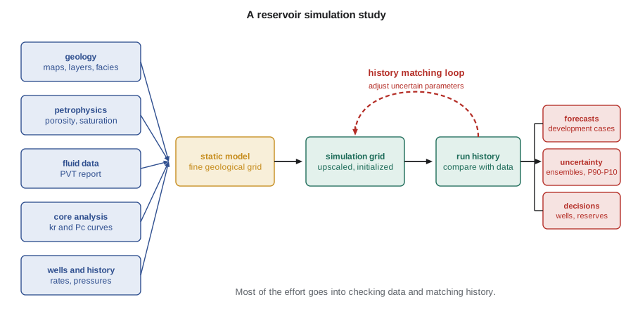
The simulation study
Lena sketches the steps of a study on the whiteboard, and they match the workflow in the figure. The first step is to define the questions. A model built to choose between two development plans needs a different level of detail from one built to estimate reserves or to design a single injector. Lena's questions are specific: which producers to convert to injectors, how much incremental oil a full-field flood will deliver, how much water must be handled and how sensitive the answer is to the thief layer. Every later decision, from grid size to the number of history match parameters, should serve those questions.
The second step is data gathering and review. The geologist supplies the structure maps, the layering and the facies model. The petrophysicist supplies porosity, water saturation and net pay from logs, calibrated to core. The fluid laboratory supplies the PVT report. Special core analysis provides relative permeability and capillary pressure. Production engineers supply well histories, completion intervals, production and injection volumes and pressure surveys. Ethan's first job is to collect and check all of it, which Lena warns him will take longer than he expects.
The third step is building the static model, a fine-scale geological description of the pool, often with millions of cells, built in a geomodelling package. The fourth step is to construct the dynamic simulation grid, usually coarser, and to upscale the static properties onto it. The fifth is initialization: placing the fluids in the model in gravity-capillary equilibrium so that the starting oil in place matches the volumetric and material balance estimates. The sixth is history matching, adjusting uncertain parameters until the model reproduces the observed pressures, rates and water cuts. The seventh is forecasting: running the matched model forward under different development plans and with different realizations of the uncertain parameters. The last is to document the study and turn the results into decisions.
| Study step | Typical share of effort | Main output |
|---|---|---|
| Define objectives and scope | Small | Questions the model must answer |
| Gather and check data | Large | Reviewed data set and known gaps |
| Static model and upscaling | Large | Simulation grid with properties |
| Initialization | Small | Equilibrated model with checked volumes |
| History matching | Largest | Calibrated model and parameter ranges |
| Forecasting and uncertainty | Medium | Cases, ranges and recommendations |
| Documentation | Medium | Report that another engineer can reproduce |
Kinds of simulator
Simulators are classified by the fluid description they use. A black-oil simulator, the workhorse of the industry, describes the hydrocarbons as two pseudo-components, stock-tank oil and surface gas, whose split between the oil and gas phases follows the solution gas-oil ratio and formation volume factors from a standard PVT report. Water is a third component that stays in its own phase. Black-oil models suit most waterfloods, depletion studies and many gas-injection studies where the fluids do not change composition much. The Cardium A pool model will be a black-oil model.
A compositional simulator tracks several hydrocarbon components, typically six to fifteen lumped groups, and uses an equation of state to split them between the phases at each block's pressure and temperature. It is needed for gas condensates, volatile oils, miscible gas or carbon dioxide injection and other processes where the composition of the phases changes as the process proceeds. Thermal simulators add an energy balance and temperature-dependent properties and are used for steam processes in heavy oil and bitumen. Other specialized models handle naturally fractured reservoirs with dual porosity, chemical floods with polymer or surfactant, coalbed methane and geological storage of carbon dioxide.
Many commercial and open-source codes are in use. Computer Modelling Group, based in Calgary, sells the IMEX black-oil, GEM compositional and STARS thermal simulators, which are widely used in heavy oil and in Canadian and international operations. SLB markets Eclipse and the newer Intersect simulator, tNavigator is another commercial package and OPM Flow is an open-source simulator developed by the Open Porous Media initiative that reads input in a widely used industry format. The MATLAB Reservoir Simulation Toolbox, MRST, is an open-source research and teaching platform. The equations inside all of them are the ones this course derives; the differences lie in numerical methods, physics options, speed, user interfaces and workflow integration.
What a simulation can and cannot tell you
A simulation model is a calculation, not a measurement. Its answers are only as good as the description of the reservoir it is given, and that description is always incomplete. Wells sample a tiny fraction of the rock: in a pool developed on 40-acre spacing, the cores and logs see perhaps one part in a million of the reservoir volume. Everything between wells is inferred from geology, seismic and the behaviour of the wells themselves. Two models that match the same history can give quite different forecasts, a problem called non-uniqueness that Lesson 10 examines in detail.
Lena's rule of thumb is that a model is most reliable when it is asked about something similar to what it has already been matched against. Asking the pilot model how a fifth producer in the same pattern will respond is a modest extrapolation. Asking it to predict a gas injection scheme across the whole pool, when it has only seen eighteen months of waterflood in one corner, is a much larger one. The engineer's job is to know which questions are which and to express the uncertainty honestly, usually with a range of outcomes rather than a single number.
Simulation also has a practical cost. A large model can take hours or days to run, and a history match may need hundreds of runs. Good studies therefore use the simplest model that can answer the question. Sector models of part of a field, two-dimensional cross sections and single-well radial models are all legitimate tools. Lena plans to start with a cross-section through the injector and two producers to understand the thief layer before building the full pilot-area model.
Worked problem
Choosing the right tool
For each question, choose between a material balance, an analytical waterflood calculation and a simulation model: (a) estimating the original oil in place from pressure and production history; (b) estimating the oil recovery at water breakthrough in a uniform linear flood; (c) predicting which of four pilot producers will water out first when the injector is completed in all layers and one layer has much higher permeability.
Show solution
- (a) The material balance needs only average pressure, production and PVT data and gives oil in place directly. It is the right first tool, and a simulator should later reproduce its answer.
- (b) The Buckley-Leverett and Welge method answers this exactly for a uniform linear system with given relative permeabilities. A simulator would give almost the same answer at much more cost, and with some numerical smearing.
- (c) This depends on layering, the location of the high-permeability layer, distances to each producer and the completion intervals. Only a model with layers and areal geometry can represent all of these together.
Answer: Use the material balance for (a), the analytical method for (b) and a simulation model for (c). Each tool also checks the others: the simulation should agree with the material balance on oil in place and with Buckley-Leverett on a uniform case.
Common mistakes
MistakeTreating a simulation result as a measurement.
InsteadIt is a calculation from an incomplete description; report it with its assumptions and a range.
MistakeBuilding the most detailed model possible before defining the questions.
InsteadDefine the questions first; they decide the grid, the physics and the effort.
MistakeSkipping the data review to get to the model sooner.
InsteadMost problems found during history matching trace back to data errors that a review would have caught.
MistakeAssuming a matched model forecasts well.
InsteadA history match is necessary but not sufficient; several different models can match the same history.
Summary and key terms
- A reservoir simulator divides the reservoir into blocks and solves a mass balance for each fluid in each block, connected by Darcy's law.
- It answers questions about where and when fluids move that tanks and analytical methods cannot.
- Each time step requires the solution of a large nonlinear system, usually by Newton's method with an iterative linear solver.
- A study runs from objectives and data review through static modelling, upscaling, initialization, history matching and forecasting.
- Black-oil, compositional and thermal simulators differ in the fluid and energy descriptions they use.
- Simulation results are uncertain and non-unique, so they should be reported as ranges and checked against simpler methods.
- Reservoir simulation
- Numerical solution of the flow equations for a reservoir divided into blocks, stepped forward in time.
- Grid block
- One of the small volumes, also called a cell, into which a simulation model divides the reservoir.
- Black-oil model
- A fluid description with stock-tank oil, surface gas and water components related by PVT tables.
- Compositional model
- A fluid description that tracks several hydrocarbon components with an equation of state.
- History matching
- Adjusting uncertain model parameters until the model reproduces observed field performance.
- Static model
- A fine-scale geological description of the reservoir properties, before flow simulation.
- Non-uniqueness
- The existence of several different models that match the same observed history.
Practice problems
Work each problem on paper first, then reveal the answer to check.
Why does a simulation model contain many small material balances?
Show answer
Each grid block has its own mass balance for each component, linked to its neighbours by Darcy flow.
When is a compositional model needed instead of a black-oil model?
Show answer
When phase compositions change significantly, as in gas condensates, volatile oils and miscible or carbon dioxide injection.
Why should a simulator be checked against the material balance?
Show answer
Both must agree on oil in place and average pressure behaviour; disagreement points to a data or model error.
What is a sector model?
Show answer
A model of part of a field, used to study a pattern or process at lower cost than a full-field model.
Lesson quiz · 5 questions
Score 60% or more to complete this lesson.
Create a free account to save your progress, take quizzes and earn a certificate.