
PET-420 · Lesson 5 of 12 · 20 min
Solving the equations: Newton-Raphson and linear solvers
An implicit time step leaves the simulator with a set of equations, one or more per block, in which the unknown new pressures and saturations appear inside nonlinear functions: formation volume factors, viscosities, relative permeabilities and capillary pressures. A million-block black-oil model has three million such equations in each time step. This lesson describes how simulators solve them: Newton-Raphson iteration for the nonlinearity and iterative linear solvers for the large sparse systems that each Newton iteration produces. Between them, these two pieces take most of the computing time in any simulation run, and most of the convergence problems an engineer meets trace back to one of them.
Residuals
Write the discretized mass balance of every component in every block so that the right-hand side is zero. The left-hand side, evaluated at a guess of the new unknowns, is called the residual. For the oil component in block i of a black-oil model it is the accumulation over the step, minus the sum of the oil flows in from the neighbours, minus the well source, all at the guessed values:
Here x is the vector of all unknowns, the sum runs over the neighbours j of block i, T_ij is the transmissibility of each connection and Φ is the phase potential, pressure corrected for depth. The mobility is evaluated at the upstream block of each connection, the one from which fluid is flowing, for reasons explained in Lesson 9. A solution of the time step is a vector x for which every residual is zero, or in practice small enough. Residuals have a direct physical meaning: a residual of 1 m³ (6 bbl) per day in a block means that the guessed state fails to conserve that much oil in the block. Convergence tolerances are usually set relative to the pore volume of the block, so that a residual is judged against what the block can hold.
Newton-Raphson iteration
Newton's method linearizes the residuals around the current guess. If x^k is the guess after k iterations, the residual at a nearby point is approximately R(x^k) + J δx, where J is the Jacobian matrix of partial derivatives of every residual with respect to every unknown. Setting this approximation to zero gives the Newton update:
Each iteration therefore requires assembling the Jacobian and solving a linear system with it. Because each residual depends only on its own block and its neighbours, the Jacobian is sparse, with the same pattern of non-zero entries as the transmissibility matrix of Lesson 3, but with a small dense block, three by three in a black-oil model, at each position. When the guess is close to the solution, Newton's method converges quadratically: the number of correct digits roughly doubles with every iteration. When the guess is far away, it can overshoot, oscillate or diverge.
The code below applies Newton's method to a small nonlinear problem: gas flow along a row of six blocks, in which the flow between blocks depends on the difference of the squares of the pressures, as it does for an ideal gas at moderate pressure. One block contains a gas source. The Jacobian is tridiagonal, so each Newton update is solved with the Thomas algorithm.
# Newton-Raphson on a nonlinear 1D gas-flow problem: flow depends on p squared
SI = True
n = 6                         # interior blocks between two fixed-pressure faces
pL, pR = 15000.0, 6000.0      # kPa
# gas flux between neighbours ~ T * (p_i^2 - p_j^2); with a source of gas in block 3
T = [1.0e-6] * (n + 1)        # face coefficients (same units), outer faces included
src = [0, 0, 120.0, 0, 0, 0]  # source term in block 3 (consistent units)
def residual(p):
    full = [pL] + p + [pR]
    return [T[i] * (full[i] ** 2 - full[i + 1] ** 2) - T[i + 1] * (full[i + 1] ** 2 - full[i + 2] ** 2) + src[i]
            for i in range(n)]
def jacobian(p):                # tridiagonal: dR_i/dp_{i-1}, dR_i/dp_i, dR_i/dp_{i+1}
    full = [pL] + p + [pR]; lo, di, up = [0.0] * n, [0.0] * n, [0.0] * n
    for i in range(n):
        x = full[i + 1]
        di[i] = -2 * T[i] * x - 2 * T[i + 1] * x
        if i > 0: lo[i] = 2 * T[i] * full[i]
        if i < n - 1: up[i] = 2 * T[i + 1] * full[i + 2]
    return lo, di, up
def thomas(a, b, c, d):
    b, d = b[:], d[:]
    for i in range(1, len(b)): w = a[i] / b[i - 1]; b[i] -= w * c[i - 1]; d[i] -= w * d[i - 1]
    x = [0.0] * len(b); x[-1] = d[-1] / b[-1]
    for i in range(len(b) - 2, -1, -1): x[i] = (d[i] - c[i] * x[i + 1]) / b[i]
    return x
p = [10000.0] * n             # first guess
f, u = (1, "kPa") if SI else (0.145038, "psia")
for it in range(8):
    R = residual(p); norm = max(abs(r) for r in R)
    print(f"iteration {it}: max residual {norm:9.3e}")
    if norm < 1e-6: break
    dp = thomas(*jacobian(p), [-r for r in R])
    p = [a + b for a, b in zip(p, dp)]
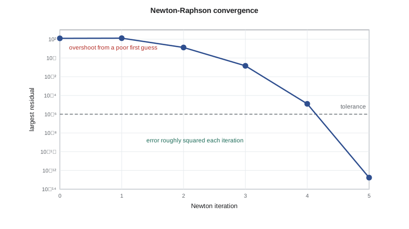
print("converged pressures:", " ".join(f"{x * f:.0f}" for x in p), u)iteration 0: max residual 1.250e+02 iteration 1: max residual 1.301e+02 iteration 2: max residual 1.309e+01 iteration 3: max residual 1.464e-01 iteration 4: max residual 1.280e-05 iteration 5: max residual 1.705e-13 converged pressures: 16327 17554 18701 16471 13887 10697 kPa
The output shows typical behaviour. From a poor first guess of uniform pressure, the first update overshoots and the residual barely changes. After that the iterations settle into the quadratic regime: the residual falls from about 10¹ to 10⁻¹, then to 10⁻⁵ and then to the limit of machine precision, roughly squaring the error at each step. A well-behaved field model converges in three to six Newton iterations per time step. Lena tells Ethan to watch the iteration counts in the run log as closely as the results themselves.
Keeping Newton on track
Field models are far less tidy than the example. Relative permeability curves have kinks at the endpoints, phases appear and disappear, wells switch between rate and pressure control and capillary pressure can be very steep near residual saturations. Each of these can make the Newton update poor. Simulators therefore limit the change allowed in a single iteration, for example to 2,000 kPa (300 psi) in pressure and 0.2 in saturation, a technique called chopping or damping. Some use line searches, which scale the update until the residual decreases. If convergence still fails within a set number of iterations, typically ten to twenty, the simulator abandons the step and retries with a shorter one.
The tolerances themselves matter. Too loose, and the accumulated mass balance error grows over thousands of steps until oil in place no longer matches production. Too tight, and the simulator spends iterations polishing digits that the data cannot justify. Default values in commercial codes are reasonable for most cases. When a model needs non-default tolerances to run, it is worth asking why.
Linear solvers
Inside each Newton iteration lies the linear system J δx = −R. For a small model, a direct solver based on Gaussian elimination is fine. For a large three-dimensional model, direct elimination fills in many of the zero entries of the sparse matrix and needs far more memory and time than the matrix itself. Simulators therefore use iterative solvers, which start from a guess of δx and improve it until the linear residual is small enough.
The standard iterative method for the nonsymmetric matrices of reservoir simulation is a Krylov subspace method, most often GMRES (generalized minimal residual) or ORTHOMIN, an older method with a similar idea that was developed for reservoir simulation. These methods build up the solution from repeated multiplications of the matrix by vectors and converge fast only when the matrix is well conditioned. Reservoir matrices are not: permeability can vary by several orders of magnitude, and the pressure and saturation parts of the system behave very differently. A preconditioner, an approximate inverse that is cheap to apply, transforms the system into one the Krylov method can solve in a few tens of iterations.
Common preconditioners include incomplete LU factorization (ILU), which performs Gaussian elimination but discards most of the fill-in, and nested factorization, long used in commercial black-oil codes. The constrained pressure residual (CPR) method is now standard for fully implicit models. It extracts the pressure part of the system, which carries the long-range elliptic character, and solves it well, often with algebraic multigrid, then cleans up the remaining local errors with a cheap method such as ILU. A good CPR preconditioner keeps the number of linear iterations nearly constant as the model grows, which is essential for models with tens of millions of cells.
| Component | What it does | Typical choice |
|---|---|---|
| Newton-Raphson | Linearizes the nonlinear residuals each iteration | Three to six iterations per step, with chopping |
| Jacobian assembly | Computes derivatives of every residual | Analytical derivatives or automatic differentiation |
| Krylov solver | Solves the sparse linear system iteratively | GMRES or ORTHOMIN |
| Preconditioner | Makes the linear system easy to solve | CPR with algebraic multigrid and ILU |
| Parallel decomposition | Splits the grid among processors | Domain decomposition with message passing |
Parallel and accelerated computing
Large models are run on many processors at once. The grid is divided into domains, each assigned to one processor, and the processors exchange the values in the blocks along domain boundaries at each linear iteration. Good domain decomposition balances the active cells and wells across processors and keeps the boundaries short. Several modern simulators also run on graphics processing units, which suit the many simple, similar operations of matrix-vector products and preconditioners. For the engineer, parallel computing mainly changes what is practical: ensembles of hundreds of models, which Lessons 10 and 11 rely on, become affordable.
Lena's pilot-area model is small by modern standards, about 150,000 active cells, and runs on a workstation in a few minutes. She still checks the solver statistics after every run: total Newton iterations, linear iterations per Newton iteration, time step cuts and the cumulative mass balance error. 'When a run that used to take five minutes suddenly takes fifty,' she says, 'the solver is usually telling you that something in the model changed, not that the computer got slower.'
Worked problem
Quadratic convergence
A Newton sequence gives largest residuals of 13.1, 0.146 and 1.28 × 10⁻⁵ at successive iterations. Show that the convergence is quadratic and estimate the next residual.
Show solution
- For quadratic convergence, each residual is roughly proportional to the square of the previous one: R_{k+1} ≈ C R_k².
- From the first pair, C ≈ 0.146 / 13.1² ≈ 8.5 × 10⁻⁴. From the second pair, C ≈ 1.28 × 10⁻⁵ / 0.146² ≈ 6.0 × 10⁻⁴. The two estimates are similar, which confirms quadratic convergence.
- The next residual is about 7 × 10⁻⁴ × (1.28 × 10⁻⁵)² ≈ 1 × 10⁻¹³, at the limit of double-precision arithmetic.
Answer: The constant C is nearly the same for both pairs, so the convergence is quadratic, and the next residual should be about 10⁻¹³, as the code output shows.
Reading solver diagnostics
Simulators report detailed solver statistics for every run, and learning to read them is part of the craft. The total number of Newton iterations divided by the number of time steps shows how hard each step was. Linear iterations per Newton iteration show how well the preconditioner is working. The number and location of time step cuts show where the trouble is. Many simulators also report the blocks or wells with the largest residuals at each failed iteration, which points directly at the source of a problem.
Ethan finds a typical example in the first pilot model. A run that should take five minutes takes forty, with hundreds of cuts. The diagnostic output names the same group of blocks again and again: a handful of tiny cells at the edge of a fault, where the corner-point geometry has created slivers with almost no pore volume. A sliver with a large transmissibility to its neighbours empties or fills completely in a fraction of a day, and its saturation swings wildly between iterations. Setting a minimum pore volume below which cells are made inactive, and reconnecting the neighbours across them, removes the problem, and the run time falls back to five minutes. The solver was never at fault; it was reporting a grid problem as clearly as it could.
Common mistakes
MistakeTreating a converged step as proof that the model is correct.
InsteadConvergence only means the discrete equations are satisfied; the data can still be wrong.
MistakeLoosening tolerances to make a model run.
InsteadFind the cause of poor convergence first; loose tolerances accumulate mass balance error.
MistakeIgnoring linear iteration counts.
InsteadA rising count signals a poorly conditioned system, often from extreme property contrasts or tiny cells.
MistakeAssuming more processors always means a faster run.
InsteadCommunication and load imbalance limit speed-up, especially for small models.
Summary and key terms
- An implicit time step requires solving nonlinear residual equations, one per component per block.
- Newton-Raphson linearizes the residuals with the Jacobian and converges quadratically near the solution.
- Chopping, line searches and time step cuts keep Newton iterations from diverging in difficult cases.
- The Jacobian is large and sparse, so it is solved with preconditioned Krylov methods such as GMRES.
- The CPR preconditioner treats the pressure part of the system separately, often with algebraic multigrid.
- Solver statistics, such as iteration counts and time step cuts, are an important diagnostic of model health.
- Residual
- The amount by which a discretized mass balance is not satisfied at a trial solution.
- Jacobian
- The matrix of derivatives of all residuals with respect to all unknowns.
- Quadratic convergence
- Convergence in which the error is roughly squared at each iteration.
- Chopping
- Limiting the change in unknowns allowed in one Newton iteration.
- Krylov method
- An iterative linear solver that builds the solution from repeated matrix-vector products.
- Preconditioner
- An approximate inverse used to make a linear system easier for an iterative solver.
- CPR
- Constrained pressure residual, a two-stage preconditioner that solves the pressure part separately.
Practice problems
Work each problem on paper first, then reveal the answer to check.
What does a residual physically represent?
Show answer
The mass of a component that the trial solution fails to conserve in a block over the step.
Why is the Jacobian sparse?
Show answer
Each residual depends only on its own block and its neighbours.
What happens when Newton fails to converge in the allowed iterations?
Show answer
The time step is cut, usually by half, and repeated.
Why is a preconditioner needed?
Show answer
Reservoir matrices are poorly conditioned, so Krylov methods converge slowly without one.
Lesson quiz · 5 questions
Score 60% or more to complete this lesson.
Create a free account to save your progress, take quizzes and earn a certificate.