
PET-420 · Lesson 4 of 12 · 20 min
Time stepping: explicit, implicit and IMPES
Space is only half of discretization. The simulator must also advance the solution in time, from the state at the start of a step to the state at its end. The choice of how to do this decides whether the model runs in minutes or days, and whether it runs at all. Ethan learns this the hard way. His first attempt at a pressure-transient check on the pilot, written as a quick spreadsheet, produces pressures of millions of kilopascals after a few steps. Lena looks at it and smiles. 'You have just met the stability limit,' she says. 'Every simulation engineer meets it once.'
Explicit and implicit differences in time
Take the one-dimensional diffusivity equation for a slightly compressible fluid, discretized in space as in Lesson 3. The time derivative becomes the change in pressure over the step divided by the step length Δt. The question is which pressures to use in the flow terms: those at the old time level n, which are known, or those at the new level n + 1, which are not.
The explicit scheme uses the old pressures. Each new block pressure is then given directly by a formula involving only known values:
The implicit scheme, also called backward Euler, uses the new pressures in the flow terms. The equation for each block then involves the unknown new pressures of the block and its neighbours, so all blocks must be solved together as a linear system:
The quantity η is the hydraulic diffusivity, and r is a dimensionless ratio of the time step to the time it takes a pressure disturbance to diffuse across one block. Both schemes are first-order accurate in time: halving the time step roughly halves the time error. A Crank-Nicolson scheme that averages the old and new levels is second order but can produce oscillations near sharp changes, and is rarely used for production runs.
The stability limit
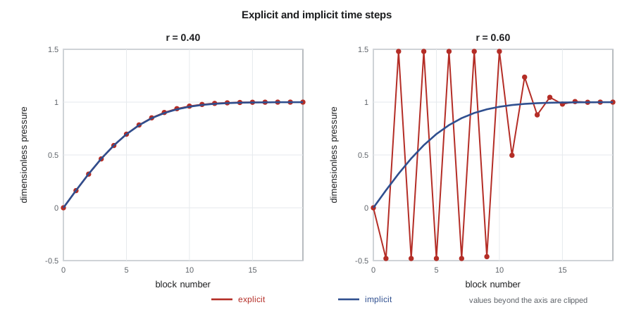
The explicit scheme is simple and cheap per step, but it is stable only if r ≤ 1/2. Above that limit, errors grow by a factor larger than one at each step, alternating in sign from block to block, until the solution is meaningless. The reason is physical: in one explicit step, information can travel only one block, and if the time step is long enough for real pressure diffusion to cross more than about one block, the scheme cannot keep up.
For reservoir rock the limit is severe. With a permeability of 15 mD, porosity 0.14, viscosity 0.72 mPa·s (0.72 cp) and total compressibility 1.5 × 10⁻⁶ per kPa (1.03 × 10⁻⁵ per psi), the diffusivity of the Cardium A pool rock is large, and for blocks 25 m (82 ft) long the explicit time step must be less than about an hour. Near a well, where blocks are small, the limit is even tighter, and it is set by the smallest and most permeable block in the whole model. Simulating twenty years of history at less than an hour per step would take hundreds of thousands of steps.
The implicit scheme has no such limit. It is unconditionally stable for the diffusion equation: errors are damped at every step whatever the step size. Large steps reduce accuracy, because the solution changes too much within one step, but the answer remains bounded and physically sensible. The code below compares the two schemes for a row of blocks drained by a well at one end.
# Explicit versus implicit time stepping for 1D slightly compressible flow (pressure diffusion)
SI = True
n, dx = 20, 25.0                 # blocks, block length (m)
k, phi, mu, ct = 15.0, 0.14, 0.72, 1.5e-6     # mD, fraction, mPa.s, 1/kPa
eta = 9.869e-16 * 1e3 / 1e-3 * 86400 * k / (phi * mu * ct)   # diffusivity, m2/d
p0, pw = 14000.0, 9000.0        # initial pressure; block 0 held at pw (a producing well)
def explicit(dt, steps):
    p = [p0] * n
    r = eta * dt / dx ** 2
    for _ in range(steps):
        new = p[:]
        for i in range(1, n - 1): new[i] = p[i] + r * (p[i - 1] - 2 * p[i] + p[i + 1])
        new[0] = pw; new[-1] = new[-2]          # no-flow outer boundary
        p = new
    return p, r
def implicit(dt, steps):
    p = [p0] * n; r = eta * dt / dx ** 2
    for _ in range(steps):
        a = [-r] * n; b = [1 + 2 * r] * n; c = [-r] * n; d = p[:]
        b[0], c[0], d[0] = 1.0, 0.0, pw; a[-1], b[-1] = -r, 1 + r
        for i in range(1, n): w = a[i] / b[i - 1]; b[i] -= w * c[i - 1]; d[i] -= w * d[i - 1]
        x = [0.0] * n; x[-1] = d[-1] / b[-1]
        for i in range(n - 2, -1, -1): x[i] = (d[i] - c[i] * x[i + 1]) / b[i]
        p = x
    return p, r
f, u = (1, "kPa") if SI else (0.145038, "psia")
dt_lim = dx ** 2 / (2 * eta)
print(f"diffusivity {eta:.0f} m2/d" if SI else f"diffusivity {eta * 10.7639:.0f} ft2/d", end="")
print(f"; explicit stability limit dt < {dt_lim * 24:.2f} h")
for dt in (0.8 * dt_lim, 1.2 * dt_lim):
    pe, r = explicit(dt, int(round(2.0 / dt)))
    pi, _ = implicit(dt, int(round(2.0 / dt)))
    print(f"dt = {dt * 24:5.2f} h (r = {r:.2f}): explicit p[5] = {pe[5] * f:12.0f} {u}, implicit p[5] = {pi[5] * f:6.0f} {u}")
pi, r = implicit(0.5, 4)
print(f"implicit with dt = 12 h (r = {r:.0f}): p[5] = {pi[5] * f:.0f} {u} after 2 days")diffusivity 8459 m2/d; explicit stability limit dt < 0.89 h dt = 0.71 h (r = 0.40): explicit p[5] = 11517 kPa, implicit p[5] = 11522 kPa dt = 1.06 h (r = 0.60): explicit p[5] = 41151067 kPa, implicit p[5] = 11535 kPa implicit with dt = 12 h (r = 7): p[5] = 11686 kPa after 2 days
Below the limit the two schemes agree closely. Just above it, the explicit result explodes to absurd values within two days, while the implicit result changes only slightly. With a twelve-hour step, about thirteen times the explicit limit, the implicit scheme still gives a reasonable answer, somewhat different from the small-step result because the large step smooths the transient. This is why pressure is always solved implicitly in reservoir simulators.
IMPES
A fully implicit black-oil simulator treats every unknown, pressure and saturations alike, implicitly. That is robust but expensive, because each Newton iteration requires solving a system with three unknowns per block. A cheaper alternative, popular since the 1960s and still used in many models, is IMPES: implicit pressure, explicit saturation.
In IMPES, the component equations are first combined to eliminate the saturation changes, giving a single pressure equation per block. That equation is solved implicitly with the mobilities from the old time level. The new pressures then give the phase flows across each face, and the saturations are updated explicitly from those flows. The method takes advantage of the different character of the two parts noted in Lesson 2: pressure is diffusive and needs implicit treatment, while saturation moves with the flow at a finite speed and can be updated explicitly if the time step is short enough.
The saturation update has its own stability limit, a form of the Courant-Friedrichs-Lewy condition. In each step, the saturation front must not move farther than about one block. In terms of the volume of fluid flowing through a block in a step compared with its pore volume, the limit is roughly:
where V_b is the bulk volume of the block, q_t is the total flow rate through it and the derivative of the fractional flow function with respect to saturation is the speed of a saturation wave relative to the total flow. The limit is tightest in small, high-throughput blocks near wells. For a typical waterflood model, IMPES time steps of a few days are possible in most of the field but can be restricted to hours by a handful of near-well blocks, which is one reason modern simulators use a mixed approach.
Fully implicit and adaptive implicit methods
The fully implicit method evaluates every term, including mobilities and fluid properties, at the new time level. Each step requires the solution of a nonlinear system by Newton's method, described in Lesson 5. It is unconditionally stable for practical purposes and allows time steps limited only by accuracy and by the convergence of the Newton iterations. Most commercial black-oil and compositional runs use it, or a variant.
The adaptive implicit method, AIM, treats each block implicitly or explicitly according to how fast it is changing. Blocks near wells and fronts, where saturations change quickly, are implicit; the large quiet regions between are explicit. This keeps most of the robustness of the fully implicit method at a cost closer to IMPES. Compositional simulators, which may have ten or more unknowns per block, benefit most.
| Method | Pressure | Saturations | Step limit | Cost per step |
|---|---|---|---|---|
| Explicit | Explicit | Explicit | Severe diffusion limit | Very low |
| IMPES | Implicit | Explicit | Saturation throughput limit | Low |
| Adaptive implicit | Implicit | Implicit where needed | Mild | Medium |
| Fully implicit | Implicit | Implicit | Accuracy and convergence only | High |
Time step control
In practice the simulator chooses its own time steps within limits set by the user. After each step it compares the largest changes in pressure and saturation in any block with target values, for example 1,000 kPa (150 psi) and 0.05 in saturation, and enlarges or shrinks the next step to bring the changes toward the targets. If the Newton iterations fail to converge, the step is cut, often by half, and repeated. Steps are also cut to land exactly on schedule events such as a well being converted to injection.
Lena shows Ethan a run log from the old full-field model. Most steps are thirty days long, but around each well event the steps drop to a fraction of a day and then grow again by a factor of two or so per step. A log full of repeated cuts is a warning sign. It usually points to a physical inconsistency, such as a well rate the reservoir cannot deliver, a block with a tiny pore volume or a discontinuous fluid table, rather than a problem with the solver itself.
Worked problem
Explicit time step limit
Estimate the explicit stability limit for blocks 25 m (82 ft) long in rock with k = 15 mD, φ = 0.14, μ = 0.72 mPa·s (0.72 cp) and c_t = 1.5 × 10⁻⁶ per kPa (1.03 × 10⁻⁵ per psi). What is the limit for blocks one fifth as long, as might be used near a well?
Show solution
- The diffusivity in metric units is η = 8.527 × 10⁻⁵ × k / (φ μ c_t) = 8.527 × 10⁻⁵ × 15 / (0.14 × 0.72 × 1.5 × 10⁻⁶) ≈ 8,460 m²/d ( (about 91,000 ft²/d)).
- The limit is Δt ≤ Δx² / (2η) = 625 / (2 × 8,460) = 0.037 d, or about 0.89 hours.
- The limit scales with Δx², so blocks one fifth as long have a limit 25 times smaller: about 2.1 minutes.
Answer: About 0.9 hours for the 25 m (82 ft) blocks and about 2 minutes for blocks one fifth as long. That is why pressure is never solved explicitly in field-scale models.
Accuracy as well as stability
Stability is only the first requirement. A stable implicit run with very long steps can still be inaccurate, because a first-order scheme smooths the solution and lags behind rapid changes. The usual check is a time step sensitivity: rerun a case with the maximum time step halved and compare the key results, such as breakthrough time, average pressure and cumulative oil. If they change by more than the uncertainty that matters for the decision, the time steps are too long. Lena runs this check once on every new model, usually on a short period around the start of injection, when the pressure and saturation changes are fastest. For the pilot model, halving the maximum step from thirty days to fifteen changed cumulative oil by less than half a percent, so the default limits were kept.
Common mistakes
MistakeSolving pressure explicitly to save effort per step.
InsteadThe diffusion limit makes explicit pressure impractically slow; solve pressure implicitly.
MistakeAssuming an implicit result is accurate because it is stable.
InsteadStability only bounds the solution; large steps still smooth transients and should be checked.
MistakeIgnoring repeated time step cuts in the run log.
InsteadFrequent cuts usually signal a data or schedule problem that should be fixed.
MistakeUsing IMPES with small near-well blocks and high rates.
InsteadThe saturation throughput limit will force tiny steps; use fully or adaptive implicit methods.
Summary and key terms
- Explicit schemes use old-level values in the flow terms; implicit schemes use new-level values and require a simultaneous solution.
- The explicit scheme for diffusion is stable only if r = ηΔt/Δx² does not exceed 1/2, which in reservoir rock means steps of minutes to hours.
- The implicit scheme is unconditionally stable for diffusion, so pressure is always solved implicitly.
- IMPES solves pressure implicitly and updates saturations explicitly, subject to a throughput limit.
- Fully implicit and adaptive implicit methods allow large stable steps at higher cost per step.
- Simulators control time steps automatically from target changes and convergence, cutting steps when Newton iterations fail.
- Explicit scheme
- A time discretization that evaluates flow terms at the old time level.
- Implicit scheme
- A time discretization that evaluates flow terms at the new time level, requiring a simultaneous solution.
- Hydraulic diffusivity
- The ratio k / (φ μ c_t), which controls how fast pressure disturbances spread.
- Stability limit
- The largest time step for which numerical errors do not grow.
- IMPES
- Implicit pressure, explicit saturation: a sequential time-stepping method.
- Adaptive implicit method
- A method that treats each block implicitly or explicitly according to how fast it changes.
- Time step cut
- Reduction and repetition of a time step after convergence failure or excessive change.
Practice problems
Work each problem on paper first, then reveal the answer to check.
Why does the explicit stability limit depend on block size squared?
Show answer
Because r = ηΔt/Δx² must stay below one half, so Δt scales with Δx².
What limits the IMPES time step?
Show answer
The saturation front must not move more than about one block per step, a throughput or CFL limit.
Why are near-well blocks the problem for time stepping?
Show answer
They are small and carry high flow rates, giving the tightest stability limits.
What does a run log with many time step cuts suggest?
Show answer
A physical or data inconsistency, such as an impossible well target or a tiny block.
Lesson quiz · 5 questions
Score 60% or more to complete this lesson.
Create a free account to save your progress, take quizzes and earn a certificate.