Exploration and seismic

The northern section that Prairie Crest is considering has no wells yet. To judge it, the geologists use data from wells on the neighbouring sections, a 3D seismic survey the company shot two winters ago and public well records filed with the AER. Ethan spends a week with the geophysicist, Nadia Petrov, learning how the seismic data were acquired and what they can and cannot show. This lesson follows the exploration toolkit from regional studies to the decision to drill, and explains why a petroleum engineer needs to understand data that someone else interprets.

From basin to prospect

Exploration narrows the search in stages. Basin analysis asks whether a sedimentary basin has the elements of a petroleum system: thick sediments, source rocks that reached the oil or gas window, reservoirs and seals. Play analysis identifies a family of similar accumulations, such as shoreline sandstones in one formation, and maps where the play works. Prospect analysis focuses on a single trap that can be drilled. At each stage the team weighs the chance of success against the size of the prize. Most exploration wells in frontier basins fail; in mature basins with good data, success rates are much higher, but the remaining prizes are smaller.

Geologists start with what can be seen and measured cheaply. Surface geology, outcrops and old well records show which rocks are present and how they are arranged. Gravity surveys detect density differences in the crust, outlining basins and salt bodies. Magnetic surveys map the depth to crystalline basement rocks, which do not hold oil. Satellite imagery and surface geochemistry can show seeps and lineaments. None of these methods images the reservoir itself; seismic reflection surveys do that, and they are the main exploration tool in almost every basin.

How seismic reflection works

A seismic survey sends sound waves into the earth and records the echoes that come back from boundaries between rock layers. On land, the source is usually a vibrator truck that shakes a steel plate against the ground with a controlled sweep of frequencies for several seconds, or a small explosive charge in a shallow drilled hole. Offshore, air guns release bursts of compressed air into the water. The returning waves are recorded by thousands of sensors called geophones on land or hydrophones at sea, laid out in lines or grids.

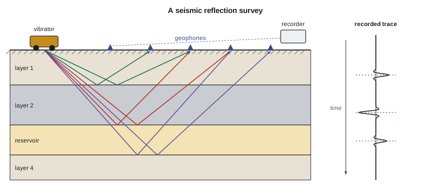
A reflection happens wherever the acoustic impedance changes. Acoustic impedance is the product of rock density and the speed of sound in the rock. When a wave meets a boundary, part of its energy reflects and part continues downward. The fraction reflected is the reflection coefficient:

Most boundaries reflect only a few percent of the energy, which is why seismic data must be recorded with sensitive instruments and processed heavily. A positive coefficient means the lower layer is harder; a negative one means it is softer. Gas in a porous sandstone lowers its velocity and density sharply, which can produce a strong negative reflection called a bright spot. Bright spots have found many gas fields, and they have also led to dry holes when low-saturation gas, which gives a similar signal, was mistaken for a commercial accumulation.

From travel time to depth

A seismic section shows reflections plotted against two-way travel time, the time for sound to go down to a reflector and back, measured in milliseconds. To drill a well, the team needs depths. The conversion uses the speed of sound in the rocks above each reflector, estimated from sonic logs and from check-shot surveys in existing wells, where a source at the surface is recorded by a tool lowered in the borehole. Depth equals velocity times half the two-way time. Because velocities change sideways as well as with depth, depth conversion is one of the largest sources of uncertainty in mapping a trap. An error of 3 percent in velocity at 2,000 m means a depth error of 60 m, which can be larger than the height of the trap itself.

# Two-way time to depth with a layered velocity model, and vertical resolution
layers = [  # name, interval velocity (m/s), two-way time at base of layer (ms)
    ('glacial drift and shale', 2200, 220),
    ('Upper Cretaceous shales', 2900, 760),
    ('Belly River sandstones', 3300, 1010),
    ('Lea Park and Colorado shales', 3500, 1150),
]
depth, t_prev = 0.0, 0
print("base of layer                    TWT (ms)   depth (m)")
for name, v, t in layers:
    depth += v * (t - t_prev) / 1000 / 2
    t_prev = t
    print(f"{name:32s} {t:6d}   {depth:8.0f}")
v_avg = depth / (t_prev / 1000 / 2)
print(f"Average velocity to {depth:.0f} m: {v_avg:.0f} m/s")
print(f"A 3 % velocity error moves this horizon by {0.03 * depth:.0f} m")

for f in (25, 40, 60):
    wavelength = 3800 / f           # sandstone interval velocity 3800 m/s
    print(f"At {f} Hz: wavelength {wavelength:5.0f} m, quarter-wave resolution {wavelength / 4:4.0f} m")

base of layer                    TWT (ms)   depth (m)
glacial drift and shale             220        242
Upper Cretaceous shales             760       1025
Belly River sandstones             1010       1438
Lea Park and Colorado shales       1150       1682
Average velocity to 1682 m: 2926 m/s
A 3 % velocity error moves this horizon by 50 m
At 25 Hz: wavelength   152 m, quarter-wave resolution   38 m
At 40 Hz: wavelength    95 m, quarter-wave resolution   24 m
At 60 Hz: wavelength    63 m, quarter-wave resolution   16 m

Seismic resolution is limited by the wavelength of the sound. The wavelength equals velocity divided by frequency, and the thinnest bed whose top and bottom can be distinguished is about a quarter of a wavelength. High frequencies resolve thin beds but are absorbed quickly by the earth, so deep targets are imaged with lower frequencies and coarser resolution. A reservoir thinner than the tuning thickness appears as a single reflection whose strength depends on the bed's thickness as well as its properties, which interpreters use cautiously to estimate thin-bed thickness.

At Tamarack Lake field, the Cardium sand bodies are only 4 to 10 m thick, thinner than the survey's quarter-wavelength resolution of about 16 to 25 m. Nadia cannot see the sands directly, but she can map the shape of the shoreline that controlled where they were deposited and use seismic attributes, mathematical measures of the reflection's amplitude and frequency, to highlight where the sand is thickest. She ties every interpretation to the well logs, because a seismic image without well control is a hypothesis, not a measurement.

2D, 3D and 4D surveys

Early surveys recorded single lines, giving 2D cross-sections through the earth. Interpreters had to guess what lay between the lines. Since the 1980s, 3D surveys have recorded closely spaced grids of sources and receivers, producing a cube of data that can be sliced in any direction. A 3D survey costs more, but it images faults, channels and reefs much more reliably and has greatly reduced the number of dry holes. Repeating a 3D survey over a producing field after several years, called 4D or time-lapse seismic, shows where fluids have moved, where water has swept the oil and where oil has been bypassed.

Most of Alberta has been covered by seismic surveys, and much of the data is owned by seismic brokerage companies that license it to producers. Surveys on farmland are usually shot in winter, when frozen ground supports the vibrator trucks and crops are not damaged. In forested areas, crews cut narrow lines through the trees. the AER and the province now require low-impact methods such as narrow, meandering lines and mulching, because old wide seismic lines fragmented the habitat of woodland caribou and other species.

Well data and the decision to drill

Wells provide direct evidence. As a well is drilled, a mud logger examines rock cuttings brought up by the drilling fluid and records gas readings. Logging tools lowered on a wireline measure resistivity, natural gamma radiation, density, neutron response and sonic velocity, from which porosity, lithology and saturation are interpreted. Cores give the most reliable data, at the highest cost. Formation testers sample fluids and measure pressures, and drill-stem tests flow the formation through the drill pipe for hours to measure its productivity. Every well, successful or not, improves the geological model for the next.

The decision to drill combines geology and economics. The team estimates the probability of geological success as the product of the chances that each element of the petroleum system is present: source, reservoir, seal, trap and timing. It then estimates the range of volumes that might be found and the value of each outcome. The expected monetary value weighs the success case against the cost of a dry hole. A prospect with a 30 percent chance of a large discovery may be worth drilling, and one with a 60 percent chance of a small one may not.

Processing and interpretation

Raw seismic records are noisy and hard to read. Processing turns them into an image. Each trace is corrected for the time it took sound to travel through the near-surface layer and for the distance between source and receiver. Traces that reflected from the same point in the subsurface are gathered and summed, a step called stacking, which strengthens the reflection and suppresses random noise. Migration moves reflections to their true positions, collapsing the diffraction patterns that faults and sharp edges produce. The result is a section or cube in which the layers appear roughly where they lie.

Interpreters then pick reflections that mark the tops of key formations, map faults and build time-structure maps, which they convert to depth with the velocity model. They tie the seismic to wells using synthetic seismograms, calculated from sonic and density logs, to confirm which wiggle corresponds to which formation top. Seismic attributes, such as amplitude, frequency content and the variation of amplitude with offset, help predict rock and fluid properties between wells. Inversion converts the reflection data into estimates of acoustic impedance, which can be related to porosity. All of these steps carry uncertainty, and good teams express their maps as ranges, not single answers.

The petroleum engineer's role is to use the interpretation wisely. Reservoir engineers turn seismic maps of structure and thickness into volumes and well locations. Drilling engineers use the depth maps to set casing points and plan well paths, and they want to know the uncertainty, because a formation coming in 30 m higher than predicted can mean a casing point in the wrong place. Completion engineers look at fault maps to avoid stimulating into faults. Asking a geophysicist how confident they are, and why, is one of the most useful habits an engineer can build.