
PET-200 · Lesson 10 of 12 · 18 min
Petroleum economics and reserves classification
In March, Prairie Crest's board must approve the year's capital budget. Lena prepares the case for the northern section: four wells at about 4.5 million dollars each, a pipeline tie-in and a battery expansion. The board will ask what the wells are worth today, how long they take to pay back, what could go wrong and how the project compares with others competing for the same money. The company's banks and shareholders will also see the result, because the new wells add to the reserves that Prairie Crest reports each year under Canadian securities rules. This lesson introduces the economics of oil and gas projects and the system used to classify and report reserves. PET-450 Petroleum Economics and Reserves Evaluation goes much further.
Cash flow
An oil and gas project is evaluated on its cash flow: the money coming in from selling oil and gas minus the money going out, year by year. Revenue is production times the price received, which is the benchmark price adjusted for quality and transport. From revenue the company pays royalties to the mineral owner, production taxes where they apply, operating costs such as power, chemicals, labour, repairs and water disposal, and income taxes. Capital costs, for drilling, completion and facilities, come at the start. Abandonment and reclamation costs come at the end. The net cash flow in each year is what the project contributes to the company.
Royalties on Crown land in Alberta are set by the province's royalty framework. New wells pay a flat 5 percent royalty until their cumulative revenue equals an allowance based on the average cost of drilling and completing a well of that depth and length; after that, a higher rate that rises with price applies. The low early rate improves the economics of expensive horizontal wells. Freehold owners negotiate their own royalties, commonly 15 to 20 percent, and the province collects a freehold mineral tax. Companies also pay municipal property taxes on wells and facilities, and the industrial carbon price on the emissions of large facilities.
Time value of money
A dollar received today is worth more than a dollar received in ten years, because it can be invested in the meantime. To compare cash flows at different times, engineers discount them back to the present at a chosen rate, which reflects the company's cost of capital and the project's risk. The net present value (NPV) is the sum of the discounted cash flows:
A project with a positive NPV at the company's discount rate adds value; a negative NPV destroys it. Oil and gas companies commonly use discount rates of 8 to 15 percent, and reserve reports present values at several rates, with 10 percent the most quoted. The internal rate of return (IRR) is the discount rate at which NPV equals zero; it measures the project's return as a percentage. Payout is the time it takes for cumulative undiscounted cash flow to turn positive. Short payouts matter in tight oil, where most of a well's value comes in its first two or three years.
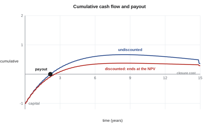
# Monthly cash flow for one new well (SI units, Canadian dollars)
qi, b, Di, Dterm = 40.0, 1.2, 1.6, 0.08      # m3/d, hyperbolic b, initial and terminal decline per year
capex, abandon = 4.5e6, 0.15e6               # dollars at month 0 and at end of life
opex_fixed, opex_var = 7500.0, 60.0          # dollars per month, dollars per m3
royalty_pre, royalty_post, allowance = 0.05, 0.25, 4.0e6   # Crown royalty 5 % until revenue reaches allowance
tax = 0.23                                    # combined income tax on positive cash flow, simplified
months, econ_limit = 360, 1.0                 # m3/d

def rate(t_years):
    D = Di / (1 + b * Di * t_years)           # current hyperbolic decline
    if D > Dterm:
        return qi / (1 + b * Di * t_years) ** (1 / b)
    # switch to exponential at the terminal decline
    t_sw = (Di / Dterm - 1) / (b * Di)
    q_sw = qi / (1 + b * Di * t_sw) ** (1 / b)
    return q_sw * 2.718281828 ** (-Dterm * (t_years - t_sw))

def evaluate(price, rate_disc=0.10):
    cum_rev, cum_cash, npv, payout, prod, flows = 0.0, -capex, -capex, None, 0.0, [-capex]
    for m in range(1, months + 1):
        q = rate((m - 0.5) / 12)
        if q < econ_limit:
            break
        vol = q * 30.4
        rev = vol * price
        roy = rev * (royalty_pre if cum_rev < allowance else royalty_post)
        cum_rev += rev
        cash = rev - roy - opex_fixed - opex_var * vol
        cash -= max(cash, 0) * tax
        prod += vol
        flows.append(cash)
        cum_cash += cash
        npv += cash / (1 + rate_disc) ** (m / 12)
        if payout is None and cum_cash > 0:
            payout = m
    flows.append(-abandon)
    npv -= abandon / (1 + rate_disc) ** ((m + 1) / 12)
    return npv, payout, prod, m, flows

def irr(flows):
    lo, hi = 0.0, 10.0          # search positive rates only
    for _ in range(200):
        mid = (lo + hi) / 2
        v = sum(f / (1 + mid) ** (i / 12) for i, f in enumerate(flows))
        lo, hi = (mid, hi) if v > 0 else (lo, mid)
    return mid

for price in (440, 530, 620):                 # dollars per m3 (about 70, 84 and 99 per barrel)
    npv, payout, prod, life, flows = evaluate(price)
    print(f"price {price} $/m3: NPV10 {npv / 1e6:5.2f} M$, IRR {irr(flows):5.0%}, payout {payout} months, "
f"EUR {prod:,.0f} m3 over {life / 12:.0f} years")price 440 $/m3: NPV10 0.63 M$, IRR 16%, payout 49 months, EUR 39,999 m3 over 25 years price 530 $/m3: NPV10 1.93 M$, IRR 30%, payout 30 months, EUR 39,999 m3 over 25 years price 620 $/m3: NPV10 3.23 M$, IRR 47%, payout 22 months, EUR 39,999 m3 over 25 years
The program shows the shape of tight-oil economics: a large negative cash flow at the start, payout within two to four years at most prices and a long tail of smaller cash flows. It also shows how sensitive the answer is to price. Engineers run sensitivities on price, costs, initial rate and decline, and present the results as a tornado chart that ranks which uncertainty matters most. In most tight-oil evaluations, oil price and initial rate dominate.
Reserves and resources
Reserves are estimated quantities of oil and gas that are expected to be recovered commercially from known accumulations, from a given date forward, under defined conditions. Each word matters. Commercially means a project to recover them must be economic, approved or reasonably certain to be approved, with access to markets. Known accumulations means they have been discovered by wells. Defined conditions means the price, cost and regulatory assumptions are stated. Oil that has been discovered but is not yet commercial, perhaps because there is no pipeline or the price is too low, is classified as contingent resources. Oil that has not been discovered but is expected from mapped prospects is prospective resources.
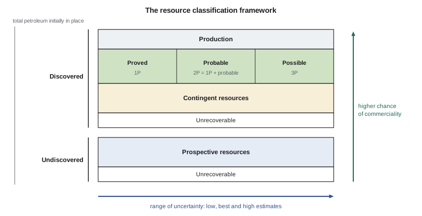
Within reserves, the categories describe uncertainty. Proved reserves (1P) are those that can be estimated with reasonable certainty; when probabilistic methods are used, there should be at least a 90 percent chance that the quantity actually recovered will equal or exceed the estimate. Probable reserves are additional quantities that are as likely as not to be recovered; proved plus probable (2P) has at least a 50 percent chance. Possible reserves are less likely still; proved plus probable plus possible (3P) has at least a 10 percent chance. Reserves are also split by development status: proved developed producing, proved developed non-producing and proved undeveloped, which need new wells or major spending.
The framework most companies follow is the Petroleum Resources Management System (PRMS), maintained by the Society of Petroleum Engineers with other professional societies. Its most recent full edition dates from 2018, with application guidelines updated since. National securities regulators set the rules for what public companies must disclose, and they build on PRMS concepts with important differences.
In Canada, National Instrument 51-101 sets the standards. Producers must file an annual statement of reserves data (Form 51-101F1), a report from an independent qualified reserves evaluator or auditor (Form 51-101F2) and a report from management and directors (Form 51-101F3). Proved and probable reserves must both be disclosed, with net present values at several discount rates, usually using forecast prices from the evaluator. Estimates must follow the Canadian Oil and Gas Evaluation Handbook (COGEH), maintained by the Society of Petroleum Evaluation Engineers (Calgary chapter); its recent updates clarified how carbon tax credits are treated in evaluations and revised the definitions of qualified evaluators and auditors.
| Feature | Canada: NI 51-101 and COGEH | United States: SEC rules |
|---|---|---|
| Required categories | Proved and probable | Proved (probable and possible optional) |
| Price basis | Forecast prices (constant prices optional) | 12-month average first-of-month price, held flat |
| Evaluator | Independent qualified reserves evaluator or auditor | Company engineers; independent audit common but not required |
| Undeveloped reserves | Must be supported by development plans | Generally drilled within five years |
| Value disclosure | NPV at several discount rates, before and after tax | Standardized measure at 10 percent |
Worked problem
Present value of a well
A Tamarack Lake field well costs 4.5 million dollars at time zero. Its net cash flows after royalties, operating costs and taxes are forecast as 2.4, 1.3, 0.9, 0.7 and 0.6 million dollars in years 1 to 5. At a 10 percent discount rate, what is its NPV over these five years, and when does it pay out?
Show solution
- Discount factors: 0.909, 0.826, 0.751, 0.683, 0.621.
- Present values: 2.18 + 1.07 + 0.68 + 0.48 + 0.37 = 4.78 million dollars.
- NPV = 4.78 − 4.5 = 0.28 million dollars.
- Cumulative cash: −4.5, −2.1, −0.8, +0.1, so payout comes late in year 3.
Answer: An NPV of about 0.28 million dollars over five years: positive but thin. The later tail of production adds more value, and abandonment cost reduces it; both must be included before the decision.
Price assumptions and risk
No input to an economic evaluation is more uncertain than price. Oil prices have swung from under 20 dollars to over 140 dollars a barrel within a few years, and gas prices are just as volatile. Companies use a planning price deck, often a set of forecasts from independent evaluators, and test projects at low and high cases. Many producers hedge part of their production for the next year or two with futures, swaps or options, locking in prices that protect their cash flow and capital program. Lenders base their credit limits on the value of a company's reserves at conservative prices, so a price collapse can shrink a company's borrowing capacity just when it needs cash.
Other risks are also built into the analysis. Geological risk, the chance that a well is poorer than expected, is handled with chances of success and ranges of outcome. Cost overruns, delays in pipeline access, regulatory changes, carbon costs and abandonment liabilities all affect value. Comparing projects on risked NPV, NPV per dollar invested and payout lets managers build a portfolio that balances quick returns, long-life production and exposure to price.
Common mistakes
MistakeAdding cash flows from different years without discounting.
InsteadDiscount each year's cash flow to the present before adding; payout is the only common measure that is undiscounted.
MistakeCalling all discovered oil reserves.
InsteadOnly commercial, approved or reasonably certain projects count as reserves; the rest is contingent resources.
MistakeTreating proved reserves as the most likely outcome.
InsteadProved is a high-confidence, low estimate; 2P is closer to the best estimate.
MistakeUsing today's spot price for US proved reserves.
InsteadThe SEC requires the 12-month average of first-day-of-the-month prices, held flat.
Summary and key terms
- Project value comes from cash flow: revenue less royalties, taxes, operating costs, capital and abandonment.
- NPV discounts each year's cash flow; IRR is the rate at which NPV is zero; payout is when cumulative cash turns positive.
- Reserves are commercial, discovered and stated under defined conditions; contingent and prospective resources are not reserves.
- 1P, 2P and 3P reflect at least 90, 50 and 10 percent chances of being met or exceeded.
- NI 51-101 requires proved and probable reserves, forecast prices, independent evaluators and COGEH methods.
- Sensitivity analysis shows which uncertainties, usually price and initial rate, matter most.
- Net present value
- The sum of a project's cash flows, each discounted to the present at a chosen rate.
- Internal rate of return
- The discount rate at which a project's net present value equals zero.
- Payout
- The time at which cumulative undiscounted cash flow becomes positive.
- Reserves
- Quantities of petroleum expected to be commercially recovered from known accumulations from a given date under defined conditions.
- Contingent resources
- Discovered quantities that are not yet commercial.
- Proved reserves
- Reserves estimated with reasonable certainty, at least a 90 percent chance of being met or exceeded.
- PRMS
- The Petroleum Resources Management System, the industry framework for classifying reserves and resources.
Practice problems
Work each problem on paper first, then reveal the answer to check.
A project costs 10 million dollars and returns 4 million dollars a year for 4 years. Find its NPV at 10 percent.
Show answer
PV = 4 × (0.909 + 0.826 + 0.751 + 0.683) = 4 × 3.170 = 12.68; NPV = 2.68 million dollars.
What is the difference between reserves and contingent resources?
Show answer
Both are discovered, but reserves are tied to a commercial, approved or reasonably certain project; contingent resources lack a condition such as a market, approval or economic viability.
An evaluator reports 1P = 2.0 million bbl and 2P = 3.1 million bbl. What are the probable reserves?
Show answer
3.1 − 2.0 = 1.1 million bbl.
Why do tight-oil projects pay out quickly but have long tails?
Show answer
Wells start at high rates and decline steeply, so most revenue comes in the first two or three years, followed by many years of low production.
Lesson quiz · 5 questions
Score 60% or more to complete this lesson.
Create a free account to save your progress, take quizzes and earn a certificate.