
MEC-210 · Lesson 2 of 12 · 27 min
Curvilinear motion: rectangular, normal-tangential and polar coordinates
Most motion is not along a straight line. A parcel leaving a chute follows a curved path, a tote on a spiral conveyor winds round a column, and the gripper of a robot arm sweeps through an arc while it extends. Describing these motions needs vectors, and it needs a coordinate system suited to the problem. This lesson develops the three systems used throughout dynamics: rectangular components, which suit projectiles; normal and tangential components, which suit motion along a known path; and polar components, which suit anything that rotates and extends at the same time. The physics is the same in all three. The choice of coordinates only decides how hard the arithmetic is.
Position, velocity and acceleration as vectors
Let the position of a particle relative to a fixed origin be the vector \(\mathbf{r}(t)\). As the particle moves, the tip of \(\mathbf{r}\) traces out the path. The velocity is the time derivative of position, \(\mathbf{v} = d\mathbf{r}/dt\), and it is always tangent to the path, pointing in the direction of motion. Its magnitude is the speed, \(v = ds/dt\), where \(s\) is the distance measured along the path.
The acceleration is \(\mathbf{a} = d\mathbf{v}/dt\). Unlike the velocity, the acceleration is generally not tangent to the path. A car going round a bend at constant speed has a velocity that is always tangent to the road, but its velocity vector is turning, and that change in direction is an acceleration pointing toward the inside of the bend. This is the single most important idea of curvilinear motion: a particle can accelerate without changing speed, simply by changing direction. Anything that follows a curve needs a force pushing it toward the inside of the curve, and the machine has to supply that force.
Rectangular components
In a fixed \(x\)-\(y\)-\(z\) frame with unit vectors \(\mathbf{i}\), \(\mathbf{j}\), \(\mathbf{k}\), the position is \(\mathbf{r} = x\mathbf{i} + y\mathbf{j} + z\mathbf{k}\). Because the unit vectors are fixed in direction, differentiating is easy:
A dot over a symbol means a derivative with respect to time. Each component behaves like an independent rectilinear motion, which is why the rectangular system is so useful when the accelerations along fixed directions are known. The classic case is projectile motion.
Projectile motion
A body moving freely near the Earth's surface, with air resistance neglected, has an acceleration of \(g\) straight down and nothing else. Taking \(x\) horizontal and \(y\) vertically up, \(a_x = 0\) and \(a_y = -g\). The horizontal motion is at constant velocity and the vertical motion is at constant acceleration:
The two motions are linked only through time. A typical problem gives enough information to find the time of flight from one direction and uses it in the other. Eliminating \(t\) shows that the path is a parabola. Parcels leaving the end of a belt, gravel thrown from a slinger conveyor, water from a nozzle and a part ejected from a press all follow nearly parabolic paths, as long as they are dense enough that air resistance is small.
Worked problem
Landing a parcel in a cart
At the end of a horizontal conveyor, parcels leave the belt and drop 0.80 m into a roll cart. The near edge of the cart opening is 0.60 m beyond the end of the belt, and the far edge is 1.00 m beyond it. What range of belt speeds will drop parcels into the cart? Treat the parcels as particles and ignore air resistance.
Show solution
- The parcel leaves horizontally, so \((v_0)_y = 0\). The fall time comes from the vertical motion: \(0.80 = \tfrac12 (9.81) t^2\), so \(t = 0.404 \text{ s}\).
- The fall time is the same for every belt speed, because the horizontal speed does not affect the vertical motion.
- Horizontal distance is \(x = v_0 t\). For the near edge, \(v_0 = 0.60 / 0.404 = 1.49 \text{ m/s}\). For the far edge, \(v_0 = 1.00 / 0.404 = 2.48 \text{ m/s}\).
Answer: Belt speeds between 1.49 and 2.48 m/s land the parcel in the cart. A real design would aim for the middle of the range and allow for parcels that slide or tumble off the end.
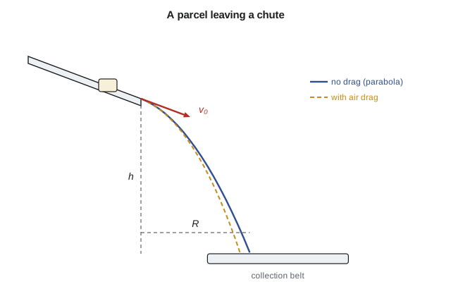
Light, bulky cartons are not dense enough to ignore air resistance completely. The program below compares the drag-free answer for a parcel leaving a sloping chute with a numerical solution that includes a drag force proportional to the square of the speed. It also computes the radius of curvature of the path at launch, which the next section explains.
# A parcel leaves the end of a chute at 3.2 m/s, angled 20 degrees below
# horizontal, 1.1 m above a collection belt. Where does it land?
# Compare the drag-free projectile answer with a numerical solution that
# includes quadratic air drag (light box, large face).
import math

g = 9.81
v0, ang, h = 3.2, math.radians(-20), 1.1
vx0, vy0 = v0 * math.cos(ang), v0 * math.sin(ang)

# Drag-free: y = h + vy0 t - g t^2/2 = 0
t_land = (vy0 + math.sqrt(vy0**2 + 2 * g * h)) / g
print(f"no drag:   flight {t_land:.3f} s, lands {vx0 * t_land:.3f} m out")

# With drag: a = -(c/m)|v| v - g j, c/m = 0.15 1/m for a light carton
cm = 0.15
dt, t, x, y, vx, vy = 1e-4, 0.0, 0.0, h, vx0, vy0
while y > 0:
    sp = math.hypot(vx, vy)
    ax, ay = -cm * sp * vx, -cm * sp * vy - g
    vx, vy = vx + ax * dt, vy + ay * dt
    x, y, t = x + vx * dt, y + vy * dt, t + dt
print(f"with drag: flight {t:.3f} s, lands {x:.3f} m out, speed {math.hypot(vx, vy):.2f} m/s")

# Radius of curvature at the start of the drag-free path: rho = v^2 / a_n
a_n = g * math.cos(ang)            # component of g normal to the velocity
print(f"radius of curvature at launch: {v0**2 / a_n:.3f} m")no drag: flight 0.375 s, lands 1.128 m out with drag: flight 0.395 s, lands 1.069 m out, speed 4.91 m/s radius of curvature at launch: 1.111 m
For this short throw, drag shortens the landing distance by about 6 cm, roughly 5 percent. That is small enough that the drag-free model is fine for a first layout, but large enough that the chute end and the receiving belt should be positioned with some adjustment. For longer throws the effect grows quickly, because drag acts for longer and the parcel is moving faster.
Normal and tangential components
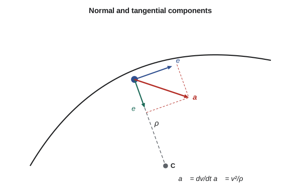
When the path is known, as it is for a vehicle on a road, a tote on a curved conveyor or a cam follower in its groove, it is natural to describe the motion relative to the path itself. At each point on the path we place two unit vectors: \(\mathbf{u}_t\), tangent to the path in the direction of motion, and \(\mathbf{u}_n\), perpendicular to it and pointing toward the centre of curvature. The velocity is purely tangential, \(\mathbf{v} = v\,\mathbf{u}_t\). The acceleration has two parts:
The tangential component, \(a_t = \dot{v}\), is the rate of change of speed. It is positive when the particle speeds up and negative when it slows down. The normal component, \(a_n = v^2/\rho\), comes from the change in direction, where \(\rho\) is the radius of curvature of the path at that point. It always points toward the centre of curvature and is never negative. On a straight line \(\rho\) is infinite and \(a_n = 0\); on a circle \(\rho\) is the radius. The magnitude of the total acceleration is \(\sqrt{a_t^2 + a_n^2}\).
For a path given as \(y = f(x)\), the radius of curvature is
Highway and railway designers use this formula to set the transition curves that ease vehicles into bends, so that the normal acceleration builds up gradually rather than jumping from zero to its full value at the start of the curve. The same thinking applies to conveyor and cam design: a sudden change in curvature means a sudden change in the force needed to hold the load on its path.
Worked problem
A tote on a curved conveyor
A tote travels round a horizontal curved section of conveyor with a centreline radius of 1.50 m. At the instant it is moving at 1.20 m/s, the drive is speeding it up at 0.40 m/s². Find the magnitude of its acceleration.
Show solution
- Tangential component: \(a_t = 0.40 \text{ m/s}^2\).
- Normal component: \(a_n = v^2/\rho = (1.20)^2/1.50 = 0.96 \text{ m/s}^2\), toward the centre of the curve.
- \[a = \sqrt{a_t^2 + a_n^2} = \sqrt{0.40^2 + 0.96^2} = 1.04 \text{ m/s}^2\]
- The acceleration points ahead of the inward normal at an angle \(\tan^{-1}(0.40/0.96) = 22.6^\circ\).
Answer: The tote accelerates at 1.04 m/s², most of it from turning. The side guides and friction must supply the inward force; Lesson 4 shows how to calculate it.
The normal acceleration grows with the square of speed. Doubling the speed of a curved conveyor quadruples the inward force needed to keep the totes on it, which is why curved sections often run slower than straight ones, or are banked.
Polar coordinates
For motion described by a distance from a fixed point and an angle, such as a robot arm that rotates about its base while its gripper slides in or out, polar coordinates are the natural choice. The position is \(\mathbf{r} = r\,\mathbf{u}_r\), where \(\mathbf{u}_r\) points from the origin toward the particle and \(\mathbf{u}_\theta\) is perpendicular to it in the direction of increasing \(\theta\). These unit vectors rotate with the particle, so their derivatives are not zero: \(\dot{\mathbf{u}}_r = \dot\theta\,\mathbf{u}_\theta\) and \(\dot{\mathbf{u}}_\theta = -\dot\theta\,\mathbf{u}_r\). Differentiating carefully gives
Each term has a physical meaning. In the radial direction, \(\ddot r\) is the acceleration of the sliding motion and \(-r\dot\theta^2\) is the centripetal acceleration of a point going round in a circle. In the transverse direction, \(r\ddot\theta\) is the acceleration due to angular acceleration, and \(2\dot r\dot\theta\) is the Coriolis acceleration. The Coriolis term appears whenever something moves outward or inward along a rotating arm. It is why a person walking outward on a turning merry-go-round feels pushed sideways, and why a robot that extends its arm while slewing feels a sideways load on the gripper that disappears if it does one motion at a time.
Worked problem
A gripper on a slewing, extending arm
A Kestrel pick robot rotates about a vertical axis at a constant rate of 1.5 rad/s. At the instant the gripper is 0.60 m from the axis, it is sliding outward along the arm at a steady 0.40 m/s. Find the acceleration of the gripper.
Show solution
- Data: \(r = 0.60 \text{ m}\), \(\dot r = 0.40 \text{ m/s}\), \(\ddot r = 0\), \(\dot\theta = 1.5 \text{ rad/s}\), \(\ddot\theta = 0\).
- \[a_r = \ddot r - r\dot\theta^2 = 0 - (0.60)(1.5)^2 = -1.35 \text{ m/s}^2\]
- \[a_\theta = r\ddot\theta + 2\dot r\dot\theta = 0 + 2(0.40)(1.5) = 1.20 \text{ m/s}^2\]
- \[a = \sqrt{1.35^2 + 1.20^2} = 1.81 \text{ m/s}^2\]
Answer: The gripper accelerates at 1.81 m/s². The radial part points in toward the axis; the transverse part is entirely Coriolis acceleration, which exists only because the gripper is moving outward while the arm turns.
A practical consequence: if the robot needs to move a delicate item, the programmer can reduce the sideways load by extending the arm and slewing it in separate phases, at the cost of a longer cycle. Many pick-and-place routines blend the motions anyway and simply limit the speeds so that the combined acceleration stays below what the gripper can hold.
Choosing a coordinate system
| Situation | Best system | Why |
|---|---|---|
| Projectiles, motion with known x and y accelerations | Rectangular | Unit vectors are fixed; components are independent |
| Motion along a known path (road, track, conveyor) | Normal-tangential | Splits speed change from direction change |
| Rotation plus radial motion (arms, slots, radar tracking) | Polar | Matches how the motion is driven or measured |
| Path given as y = f(x) and speed known | Normal-tangential, with ρ from the formula | Normal acceleration needs only v and ρ |
The three systems describe the same physical acceleration, so any one of them gives the right answer if used correctly. The test of a good choice is how many terms vanish. For the robot arm, polar coordinates make the problem a few lines long; in rectangular coordinates it would require differentiating sines and cosines of a changing angle. A minute spent choosing coordinates often saves ten minutes of algebra and avoids most sign errors.
Common mistakes
MistakeAssuming acceleration is zero when speed is constant.
InsteadA particle on a curve has normal acceleration v²/ρ even at constant speed.
MistakePointing the normal acceleration away from the centre of curvature.
InsteadIt always points toward the centre of curvature.
MistakeTreating the polar unit vectors as fixed when differentiating.
InsteadThey rotate with the particle, which produces the -rθ̇² and 2ṙθ̇ terms.
MistakeUsing a different time of flight in the horizontal and vertical projectile equations.
InsteadThe same time links the two motions.
MistakeForgetting that the velocity is always tangent to the path.
InsteadUse this to find directions and to check answers.
Summary and key terms
- Velocity is tangent to the path; acceleration generally is not.
- Rectangular components treat each direction as an independent rectilinear motion.
- Projectiles have a_x = 0 and a_y = -g, linked only by time.
- In normal-tangential components, a_t = dv/dt and a_n = v²/ρ toward the centre of curvature.
- In polar components, a_r = r̈ - rθ̇² and a_θ = rθ̈ + 2ṙθ̇.
- The Coriolis term 2ṙθ̇ appears when something moves along a rotating arm.
- Choose the coordinate system that makes the most terms vanish.
- Curvilinear motion
- Motion along a curved path.
- Projectile
- A body moving under gravity alone, with air resistance neglected.
- Radius of curvature
- The radius of the circle that best fits the path at a point.
- Normal acceleration
- The component of acceleration toward the centre of curvature, equal to v²/ρ.
- Tangential acceleration
- The component of acceleration along the path, equal to the rate of change of speed.
- Centripetal acceleration
- Acceleration toward the centre of a circular path.
- Coriolis acceleration
- The 2ṙθ̇ term that arises from radial motion along a rotating line.
- Polar coordinates
- A position described by a distance from a fixed point and an angle.
Practice problems
Work each problem on paper first, then reveal the answer to check.
A part is ejected horizontally at 2.0 m/s from a press 1.2 m above the floor. How far from the press does it land?
Show answer
t = sqrt(2 x 1.2 / 9.81) = 0.495 s; x = 2.0 x 0.495 = 0.99 m.
A tote on a circular curve of radius 2.0 m travels at a constant 1.5 m/s. What is its acceleration?
Show answer
a = a_n = 1.5²/2.0 = 1.125 m/s², toward the centre.
If the tote speed in the curved-conveyor example were doubled, what would the normal acceleration become?
Show answer
Four times as large: 3.84 m/s².
In the robot example, what is the acceleration if the arm stops extending (ṙ = 0)?
Show answer
Only the radial term remains: 1.35 m/s² toward the axis.
Change the program so the parcel leaves horizontally at 3.2 m/s. Does it land farther or closer?
Show answer
Farther, because it starts with no downward velocity and so stays in the air longer.
Find the radius of curvature of y = 0.5x² at x = 0.
Show answer
dy/dx = 0 and d²y/dx² = 1, so ρ = 1.
Lesson quiz · 5 questions
Score 60% or more to complete this lesson.
Create a free account to save your progress, take quizzes and earn a certificate.