
MBA-504 · Lesson 8 of 12 · 21 min
Simple and multiple regression
Northfield Components is preparing its budget for next year, and Daniel needs to forecast factory overhead: maintenance, utilities, indirect labour, supplies and the many other costs that are not tied to a specific part. The plant's operations plan calls for about 40,000 machine hours a month next year, more than in most recent months. In MBA-501, Professor Achterberg showed the cohort how to split a mixed cost into fixed and variable parts with the high-low method, which uses only the busiest and quietest months. Daniel wants something better, a method that uses all 24 months of data and tells him how confident he can be in the forecast. Dr. Zhou introduces regression, which she calls the workhorse of business analysis.
Fitting a line
Simple linear regression fits a straight line through a scatter of points to describe how an outcome, the dependent variable, changes with a single explanatory variable. The line has an intercept, the predicted outcome when the explanatory variable is zero, and a slope, the change in the predicted outcome for a one-unit increase in the explanatory variable. Among all possible lines, regression chooses the one that minimizes the sum of the squared vertical distances between the points and the line. This is the method of least squares, developed independently by Adrien-Marie Legendre and Carl Friedrich Gauss in the early nineteenth century to fit the orbits of comets and planets.
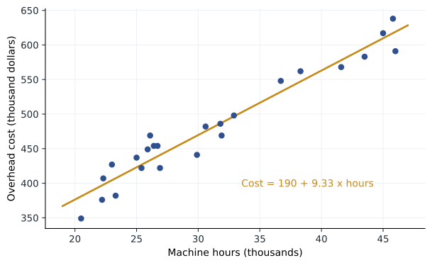
Daniel's data show monthly overhead, in thousands of dollars, against machine hours, in thousands, for the past two years. The fitted line is cost equals 189.7 plus 9.33 times machine hours. The slope says that each additional thousand machine hours is associated with about 9,330 dollars of extra overhead, an estimate of the variable overhead rate. The intercept of 189.7 thousand dollars is an estimate of fixed monthly overhead, although Daniel should be careful: the plant has never run at anywhere near zero hours, so the intercept is an extrapolation and is best read as the fixed portion within the normal operating range.
How well does the line fit?
Two numbers summarize the fit. R-squared is the share of the variation in the outcome that the line explains. Daniel's line has an R-squared of 0.94: 94 per cent of the month-to-month variation in overhead is associated with variation in machine hours. The residual standard error is the typical size of the vertical distances between the points and the line, the residuals. Here it is about 19.7 thousand dollars: actual monthly overhead typically differs from the line's prediction by about twenty thousand dollars.
A high R-squared is reassuring but not the goal. In many business settings, such as predicting sales of individual products or the behaviour of individual customers, R-squared values of 0.2 or 0.3 can be useful, while a model with an R-squared of 0.99 can be misleading if it was fitted to a trend that both variables share over time. The test of a regression is whether it answers the question it was built for, with honest uncertainty.
Uncertainty in the slope
The slope is estimated from a sample of 24 months, so it has a standard error. For Daniel's data the standard error of the slope is about 0.50, and a 95 per cent interval runs from roughly 8.3 to 10.4 thousand dollars per thousand hours. The t statistic for the slope, the estimate divided by its standard error, is about 18.7, which means the relationship is far too strong to be chance. Most software reports this alongside a p-value testing whether the slope is zero. For a cost model, that test is rarely in doubt; the interval is more useful because it shows how precisely the variable rate is known.
Predicting with honest uncertainty
To forecast overhead at 40,000 machine hours, Daniel substitutes 40 into the equation: 189.7 plus 9.33 times 40 gives about 563 thousand dollars a month. But a single month's overhead will not fall exactly on the line. A prediction interval for an individual month combines the uncertainty in the line itself with the scatter of individual months around it. For 40,000 hours it is about 563 plus or minus 43 thousand dollars, or roughly 520 to 606 thousand. The interval widens as the forecast point moves away from the average of the data, which here is about 31,000 hours, because small errors in the slope matter more far from the centre.
Daniel also notes a deeper risk. Forty thousand hours is near the top of the plant's recent experience. If the operations plan had called for 60,000 hours, the line would predict about 750 thousand dollars, but the plant would almost certainly need a third shift, more supervisors and perhaps another compressor, so overhead would jump in a way no straight line fitted to past data could capture. Regression describes relationships within the range of the data; extrapolating far beyond it is guesswork dressed up as analysis.
# Simple regression of monthly overhead on machine hours, with a prediction interval
import math, statistics
hours = [25.9, 45.0, 23.3, 38.3, 22.2, 26.4, 46.0, 25.4, 36.7, 31.9, 31.8, 32.9,
         25.0, 41.6, 22.3, 26.1, 20.5, 26.9, 30.6, 43.5, 29.9, 23.0, 26.7, 45.8]
cost = [449, 617, 382, 562, 376, 454, 591, 422, 548, 469, 486, 498,
        437, 568, 407, 469, 349, 422, 482, 583, 441, 427, 454, 638]
n = len(hours)
fit = statistics.linear_regression(hours, cost)
pred = [fit.intercept + fit.slope * h for h in hours]
sse = sum((c - p) ** 2 for c, p in zip(cost, pred))
sst = sum((c - statistics.mean(cost)) ** 2 for c in cost)
s = math.sqrt(sse / (n - 2))
sxx = sum((h - statistics.mean(hours)) ** 2 for h in hours)
se_slope = s / math.sqrt(sxx)
print(f"cost = {fit.intercept:.1f} + {fit.slope:.2f} x hours")
print(f"R-squared {1 - sse / sst:.3f}, residual std error {s:.1f}, slope SE {se_slope:.2f}")
x0, t = 40, 2.074                      # t value for 22 degrees of freedom
y0 = fit.intercept + fit.slope * x0
half = t * s * math.sqrt(1 + 1 / n + (x0 - statistics.mean(hours)) ** 2 / sxx)
print(f"Forecast at {x0}k hours: {y0:.0f}, 95% prediction interval {y0 - half:.0f} to {y0 + half:.0f}")cost = 189.7 + 9.33 x hours R-squared 0.941, residual std error 19.7, slope SE 0.50 Forecast at 40k hours: 563, 95% prediction interval 520 to 606
Multiple regression
Overhead rarely depends on one thing. Daniel's maintenance manager points out that setups, the changeovers between part numbers, drive a lot of indirect labour and scrap, and that busy months tend to involve more setups as well as more machine hours. Multiple regression extends the method to several explanatory variables at once. Each coefficient now measures the change in the outcome associated with a one-unit change in that variable, holding the other variables in the model constant. This is what makes multiple regression useful: it can separate the influence of variables that move together in the data.
To see how this works, Dr. Zhou gives the cohort a simulated version of three years of monthly data in which overhead truly depends on both hours and setups, and in which busy months have more of both. A regression on hours alone credits hours with the cost of the setups that come with them, and so overstates the variable rate per hour. Adding setups to the model brings the hours coefficient much closer to its true value and gives a separate rate per setup.
# Multiple regression by least squares, solved with the normal equations
import random, statistics
random.seed(8)
months = 36
hours = [random.uniform(20, 46) for _ in range(months)]                 # machine hours, thousands
setups = [round(2.0 * h + random.gauss(0, 10)) for h in hours]           # busier months need more setups
cost = [150 + 7.0 * h + 1.8 * s + random.gauss(0, 15) for h, s in zip(hours, setups)]

def solve(A, y):                     # Gaussian elimination for a small square system
    n = len(A); M = [row[:] + [v] for row, v in zip(A, y)]
    for i in range(n):
        p = max(range(i, n), key=lambda r: abs(M[r][i])); M[i], M[p] = M[p], M[i]
        for r in range(i + 1, n):
            f = M[r][i] / M[i][i]
            M[r] = [a - f * b for a, b in zip(M[r], M[i])]
    x = [0.0] * n
    for i in reversed(range(n)):
        x[i] = (M[i][n] - sum(M[i][j] * x[j] for j in range(i + 1, n))) / M[i][i]
    return x

X = [[1.0, h, s] for h, s in zip(hours, setups)]
XtX = [[sum(r[i] * r[j] for r in X) for j in range(3)] for i in range(3)]
Xty = [sum(r[i] * c for r, c in zip(X, cost)) for i in range(3)]
b0, b1, b2 = solve(XtX, Xty)
simple = statistics.linear_regression(hours, cost)
pred = [b0 + b1 * h + b2 * s for h, s in zip(hours, setups)]
sse = sum((c - p) ** 2 for c, p in zip(cost, pred))
sst = sum((c - statistics.mean(cost)) ** 2 for c in cost)
print(f"Hours only:       cost = {simple.intercept:6.1f} + {simple.slope:5.2f} x hours")
print(f"Hours and setups: cost = {b0:6.1f} + {b1:5.2f} x hours + {b2:4.2f} x setups")
print(f"R-squared with both variables: {1 - sse / sst:.3f}")
print(f"Correlation between hours and setups: {statistics.correlation(hours, setups):.2f}")Hours only: cost = 124.7 + 11.50 x hours Hours and setups: cost = 136.2 + 8.11 x hours + 1.47 x setups R-squared with both variables: 0.982 Correlation between hours and setups: 0.86
In the simulation, the hours-only model estimates 11.50 thousand dollars per thousand hours, well above the true rate of 7.0 used to create the data. The two-variable model estimates 8.11 per thousand hours and 1.47 per setup, much closer to the true values of 7.0 and 1.8, and explains 98 per cent of the variation. The estimates are not exact, because hours and setups are highly correlated, with a correlation of 0.86, which makes it hard for the data to separate their effects. For Daniel, the practical consequence is important. If the plant reduces setups by scheduling longer runs, the hours-only model would not predict any saving, while the two-variable model predicts roughly 1,500 dollars of overhead saved per setup avoided.
Omitted variables and collinearity
The overstated hours coefficient is an example of omitted variable bias, the regression version of the confounding discussed in lesson 7. When a variable that affects the outcome is left out of a model and is correlated with an included variable, the included variable's coefficient absorbs part of the omitted variable's effect. The bias is in the direction of the omitted variable's effect multiplied by its correlation with the included one. The only cures are to measure and include the confounder, or to find a design, such as an experiment, that breaks the link.
The opposite problem, collinearity, arises when explanatory variables are so closely related that the model cannot tell them apart. Coefficients become imprecise, can change sign when a variable is added or removed, and may look insignificant individually even though together they explain the outcome well. Collinearity does not bias predictions within the range of the data, but it makes the individual coefficients unreliable as estimates of separate effects. Collecting data in which the variables vary independently, such as months with many hours but few setups, is the best remedy.
| Output item | What it tells a manager | Common misreading |
|---|---|---|
| Coefficient | Change in the outcome per unit change in the variable, others held constant | A causal effect, regardless of design |
| Standard error and interval | How precisely the coefficient is estimated | Ignored in favour of the point estimate |
| p-value | Evidence that the coefficient differs from zero | A measure of importance |
| R-squared | Share of variation explained by the model | The main test of a good model |
| Residual standard error | Typical size of prediction errors | Overlooked, though it sets forecast accuracy |
Residuals tell you what the model missed
After fitting a model, plot the residuals against the fitted values and against each explanatory variable. If the model is adequate, the residuals should look like a shapeless cloud around zero. A curved pattern suggests the relationship is not a straight line; a funnel shape, with residuals spreading out as fitted values grow, suggests that the errors are larger for larger values, which is common with money amounts; and a pattern over time suggests that something, such as a seasonal effect or a trend, has been left out.
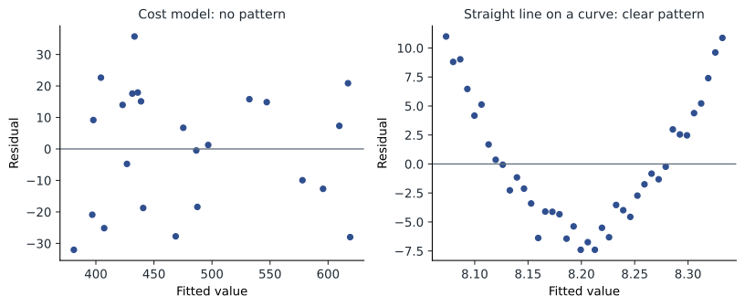
Daniel's residual plot shows no obvious pattern, which supports using the simple model for next year's budget, with the prediction interval reported alongside the point forecast. He also plans to collect setup counts for the past two years, so that next year's analysis can separate the two drivers and support the scheduling discussion.
Worked problem
Using regression to set a delivery price
Fairway's home-delivery team has data on 400 deliveries: the cost of each delivery against distance in kilometres. A regression gives cost = 6.40 + 0.85 x kilometres, with an R-squared of 0.58, a slope standard error of 0.04 and a residual standard error of 3.10 dollars. Grace wants to know the expected cost of a 12-kilometre delivery and how much a single delivery might vary.
Show solution
- Expected cost: 6.40 + 0.85 x 12 = 6.40 + 10.20 = 16.60 dollars.
- Slope interval: 0.85 plus or minus about 1.96 x 0.04, or roughly 0.77 to 0.93 dollars per kilometre, so the per-kilometre rate is precisely estimated.
- Individual variation: with a residual standard error of 3.10, an individual 12-kilometre delivery will commonly cost anywhere from about 10.50 to 22.70 dollars (plus or minus about two residual standard errors).
- Interpretation: distance explains just over half the variation; stops per route, traffic and time of day probably explain much of the rest and could be added to the model.
Answer: The average 12-kilometre delivery costs about 16.60 dollars, but individual deliveries vary widely. Grace uses the average to set a distance-based fee and asks the team to collect stop counts and time-of-day data to build a better model.
Common mistakes
MistakeThe intercept is the cost when activity is zero.
InsteadIt is often an extrapolation outside the data; read it as the fixed part within the normal range.
MistakeA high R-squared means the model is right.
InsteadModels can fit well and still be biased or useless for the decision; check residuals and design.
MistakeA regression coefficient is a causal effect.
InsteadIt is an association holding other included variables constant; omitted confounders can bias it.
MistakeForecasts from a regression are exact.
InsteadReport a prediction interval, which widens away from the centre of the data and ignores structural change.
Summary and key terms
- Least squares fits the line that minimizes the sum of squared residuals.
- The slope is the change in the outcome per unit change in the explanatory variable; check its interval.
- R-squared measures the share of variation explained; the residual standard error measures typical prediction error.
- Multiple regression separates the effects of correlated variables, holding the others constant.
- Beware omitted variable bias, collinearity and extrapolation, and always examine residual plots.
- Dependent variable
- The outcome a regression model explains or predicts.
- Least squares
- Choosing coefficients to minimize the sum of squared differences between actual and predicted values.
- R-squared
- The share of variation in the outcome explained by the model.
- Residual
- The difference between an actual value and the value predicted by the model.
- Prediction interval
- A range likely to contain an individual future value, wider than the interval for the average.
- Omitted variable bias
- Bias in a coefficient when a relevant correlated variable is left out of the model.
Practice problems
Work each problem on paper first, then reveal the answer to check.
A regression of monthly sales (thousand dollars) on advertising spend (thousand dollars) gives sales = 120 + 3.2 x advertising. Interpret the slope.
Show answer
Each additional thousand dollars of advertising is associated with about 3,200 dollars of extra monthly sales, within the range of the data; it is not necessarily causal.
Using Daniel's model, predict overhead at 30,000 machine hours.
Show answer
189.7 + 9.33 x 30 = 189.7 + 279.9, about 470 thousand dollars.
A model of store sales on store size gives a large positive coefficient. When local population is added, the size coefficient halves. Why?
Show answer
Larger stores tend to be in more populous areas; without population in the model, size absorbed part of the population effect (omitted variable bias).
A residual plot shows residuals spreading out as fitted values increase. What does this suggest?
Show answer
The errors are larger for larger values; consider modelling the logarithm of the outcome or using methods that allow unequal variance.
Lesson quiz · 5 questions
Score 60% or more to complete this lesson.
Create a free account to save your progress, take quizzes and earn a certificate.