
MBA-504 · Lesson 6 of 12 · 20 min
Comparing groups and the danger of p-hacking
Fairway Grocers ran twenty different promotions last quarter, from buy-one-get-one offers on cereal to loyalty-point bonuses on fresh produce. For each one, the analytics team compared sales in stores running the promotion with matched stores that did not, and reported the results to Grace with a p-value. Six of the twenty promotions came back statistically significant at the five per cent level, and the merchandising team wants to roll all six out across the chain. Grace's question for Dr. Zhou is whether six winners out of twenty is impressive. The answer, she learns, depends on how many of those winners chance alone would have produced.
Comparing two averages
Lesson 5 compared two proportions. Many business comparisons involve averages instead: average sales per store, average handling time, average order value. The logic is the same. The difference between two sample means is divided by its standard error to give a test statistic, and the p-value is read from a reference distribution. When the two groups may have different spreads, the safest choice is Welch's t-test, which does not assume equal variances. The standard error of the difference is the square root of the sum of each group's variance divided by its sample size.
Suppose 30 stores running a cereal promotion averaged weekly category sales of 18,400 dollars with a standard deviation of 2,600, while 30 matched stores without it averaged 17,100 with a standard deviation of 2,400. The standard error is the square root of 2,600 squared over 30 plus 2,400 squared over 30, about 646 dollars, and t is 1,300 divided by 646, about 2.0. With roughly 58 degrees of freedom, the two-sided p-value is just under 0.05. The promotion appears to have lifted sales by about eight per cent, with a 95 per cent interval running from close to zero to about 2,600 dollars a week.
Paired comparisons
A powerful way to reduce noise is to compare each unit with itself. If the same stores are measured before and after a change, or the same customers are shown both versions of something, the analysis can work with the differences within each unit. This removes the large variation between stores, such as size and location, that would otherwise swamp the effect. A paired design often needs far fewer observations than a comparison of two separate groups. Its weakness is that anything else that changed between the two periods, such as the season or a competitor's opening, is mixed in with the effect, so it works best when combined with a comparison group that did not receive the change.
The most common design in retail combines both ideas. Fairway's analysts take the change in sales from the previous period to the promotion period in the stores that ran the promotion, and subtract the change over the same weeks in matched stores that did not. This difference-in-differences approach removes both the permanent differences between stores and the common shocks that hit all stores, such as weather or a holiday. Lesson 7 returns to it as a tool for observational data.
More than two groups
When a team compares several options at once, such as three shelf layouts or four price points, it is tempting to run a test for every pair. With four groups there are six pairs, and with ten groups there are forty-five. The analysis of variance, usually shortened to ANOVA, offers a single test of whether any of the group means differ, by comparing the variation between group averages with the variation within groups. If the F statistic, the ratio of these two kinds of variation, is large, at least one group differs. Follow-up comparisons can then identify which, with adjustments for the number of comparisons made.
The multiple comparisons problem
Here lies the answer to Grace's question. If a promotion has no real effect, a test at the five per cent level will still declare it significant five per cent of the time. Test twenty promotions with no real effects, and on average one will come out significant by chance. The probability that at least one of twenty independent tests produces a false positive is one minus 0.95 to the power of 20, about 64 per cent. Six winners out of twenty is more than chance would usually produce, so some of the promotions probably work, but there is a good chance that one or two of the six are flukes.
The same problem appears whenever many comparisons are made: testing a campaign in every region, looking for differences across a dozen customer segments, checking whether an engagement survey shows significant changes on forty items, or screening hundreds of potential drivers of churn. The more places one looks, the more likely it is to find something that looks significant but is just noise.
Corrections: Bonferroni and false discovery rates
The simplest correction, named after the Italian mathematician Carlo Bonferroni, divides the significance level by the number of tests. With twenty tests at an overall level of five per cent, each test must reach a p-value below 0.0025 to count. This controls the chance of any false positive across the whole family of tests, but it is strict: when many tests are run, real but modest effects are likely to be missed.
A more forgiving approach, introduced by Yoav Benjamini and Yosef Hochberg in 1995, controls the false discovery rate instead: the expected share of declared winners that are actually false. Sort the p-values from smallest to largest and compare the k-th smallest with k divided by m, times the chosen rate. Find the largest k whose p-value falls below its threshold, and declare that test and all smaller ones significant. For a manager rolling out promotions, controlling the share of duds among the winners is often more relevant than avoiding any dud at all.
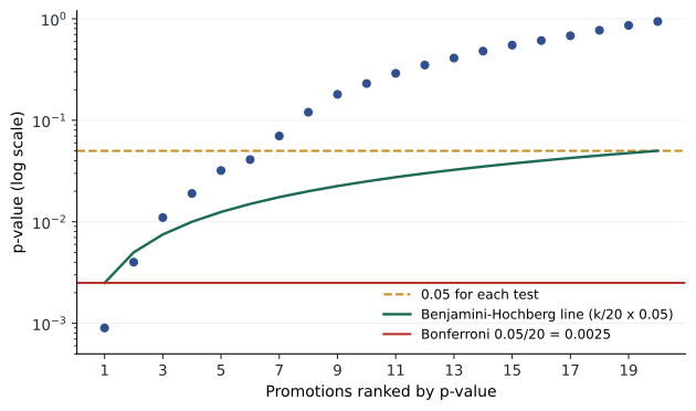
# Fairway's 20 promotion p-values under three decision rules
pvals = [0.0009, 0.004, 0.011, 0.019, 0.032, 0.041, 0.07, 0.12, 0.18, 0.23,
         0.29, 0.35, 0.41, 0.48, 0.55, 0.61, 0.68, 0.77, 0.86, 0.94]
m, alpha = len(pvals), 0.05
ranked = sorted(pvals)
unadjusted = sum(p < alpha for p in ranked)
bonferroni = sum(p < alpha / m for p in ranked)
k_bh = 0
for k, p in enumerate(ranked, start=1):
    if p <= k / m * alpha:
        k_bh = k                       # largest k passing its threshold
print(f"Unadjusted at 0.05: {unadjusted} winners")
print(f"Bonferroni at {alpha / m:.4f}: {bonferroni} winners")
print(f"Benjamini-Hochberg at a 5% false discovery rate: {k_bh} winners")
print(f"Chance of at least one false positive in {m} null tests: {1 - (1 - alpha) ** m:.0%}")Unadjusted at 0.05: 6 winners Bonferroni at 0.0025: 1 winners Benjamini-Hochberg at a 5% false discovery rate: 2 winners Chance of at least one false positive in 20 null tests: 64%
The analysis gives Grace a more defensible story. Two promotions pass the Benjamini-Hochberg threshold and are very likely to be real; one of them is strong enough to pass even Bonferroni. The other four unadjusted winners, with p-values between 0.011 and 0.041, are promising but uncertain. Grace proposes rolling out the two strong promotions now and re-testing the four borderline ones in a fresh set of stores. A promotion that wins again in a new test is far more likely to be real than one that won once among twenty.
P-hacking and the garden of forking paths
Multiple comparisons are not always visible. An analyst who tries several ways of measuring the outcome, drops a few awkward stores, adds or removes control variables, splits the data by region and stops when something reaches significance has effectively run many tests, even if only one is reported. This is p-hacking. The statisticians Andrew Gelman and Eric Loken called the subtler version the garden of forking paths: even without deliberate fishing, the many reasonable choices made after seeing the data allow analysts to find patterns that will not hold up. A related habit, hypothesizing after the results are known, presents an unexpected finding as if it had been predicted all along.
The consequences became visible in science during what is often called the replication crisis. In 2015 the Open Science Collaboration reported an attempt to repeat 100 published psychology studies; only about 36 per cent of the repeat studies produced statistically significant results, and the effects found were on average about half the size of the originals. Similar problems have been found in economics, medicine and management research. Several of the popular findings discussed in MBA-503, such as ego depletion and power posing, weakened or disappeared when tested again with larger samples. Business analytics has the same incentives, often without any peer review at all.
| Practice | Why it misleads | Safeguard |
|---|---|---|
| Testing many metrics and reporting the one that moved | Some metric will move by chance | Name one primary metric in advance |
| Slicing results by segment after the fact | Many segments mean many tests | Treat segment findings as hypotheses to re-test |
| Stopping when the result looks good | Chance crossings get locked in | Fix the sample size or use sequential methods |
| Dropping inconvenient data points | Analyst choice drives the result | Write exclusion rules before analysis |
| Reporting only successful tests | The record overstates what works | Keep a log of every test and its result |
The winner's curse
Even when a winning result is real, its size is usually overstated. Among many tests, the ones that cross the significance threshold are disproportionately those where chance pushed the estimate upwards. If Fairway picks the promotion with the largest estimated lift out of twenty, its true lift is likely to be smaller than measured. Economists call this the winner's curse, borrowing the term from auctions, where the highest bidder tends to be the one who most overestimated the item's value. Managers should expect results to shrink when a winning change is rolled out, and budgets built on the original estimate will often disappoint.
The protection is the same in every case: confirm findings on fresh data. Analysts can split historical data into an exploration set, where they search freely, and a confirmation set, held back and examined only once to test the patterns they found. For experiments, a follow-up test or a holdout group that does not receive the rolled-out change gives an honest measure of the effect at scale. Some organizations ask analysts to write a short pre-analysis plan, stating the hypothesis, metric, sample and method, before the data are examined, a practice borrowed from clinical trials.
Building a culture that tests honestly
Multiple comparisons and p-hacking are not only technical problems; they are organizational ones. Analysts respond to what managers reward. If a team is praised for finding winners and questioned only when results are disappointing, it will find winners, whether or not they are real. Dr. Zhou describes a retailer she once advised whose test log showed that more than half of its experiments had produced significant improvements, an implausibly high rate given the evidence from firms such as Microsoft that most ideas do not work. When the company re-tested a sample of its past winners, most of the improvements disappeared.
Several practices help. Keep a central register of every test, recording the hypothesis, primary metric, planned sample size and result before and after the test, so that failures are as visible as successes. Celebrate well-run tests rather than positive results, because a clean negative result saves the company from rolling out something useless. Ask for confidence intervals rather than verdicts, so that discussion focuses on the plausible size of effects. Re-test surprising or very large effects before acting on them, since surprising results are the most likely to be flukes. And give analysts the standing to say that the data do not support a conclusion, even when a senior manager hoped they would. Grace adopts a version of this at Fairway: every promotion test now begins with a one-paragraph plan filed before launch, and the merchandising team reviews the full register, including the many promotions that did nothing, at the end of each quarter.
Worked problem
Re-reading an engagement survey
Hana's annual staff survey has 40 items. The report highlights that 3 items show a statistically significant change from last year at the 5 per cent level, including a drop in agreement that managers recognize good work. Senior leaders want to launch a recognition program in response.
Show solution
- Count the tests: 40 items compared with last year gives 40 tests.
- Find the chance expectation: with no real changes, about 40 times 0.05 = 2 items would be significant on average.
- Assess the evidence: 3 significant items is close to what chance would produce, so the result is weak evidence of real change.
- Look for corroboration: check whether related items moved in the same direction, whether the drop is consistent across departments, and whether exit interviews or turnover point the same way.
Answer: Hana advises the leadership team that the recognition result may be noise and should not on its own justify a new program. She proposes tracking the item in a short pulse survey next quarter; if the drop persists and is echoed in related questions, the case for action becomes much stronger.
Common mistakes
MistakeSix significant results out of twenty means six effects are real.
InsteadAbout one false positive is expected by chance among twenty null tests; adjust for multiple comparisons.
MistakeTrying several analyses and reporting the best one is harmless exploration.
InsteadEach choice is another test; unreported choices inflate false positives.
MistakeThe measured effect of a winning test is the effect to expect at rollout.
InsteadWinners tend to be overestimated; expect shrinkage and confirm on fresh data.
MistakeBonferroni is always the right correction.
InsteadIt controls any false positive but is strict; false discovery rate control often suits business screening better.
Summary and key terms
- Compare means with Welch's t-test; use paired or difference-in-differences designs to remove noise.
- With m tests at level alpha, the chance of at least one false positive is 1 minus (1 minus alpha) to the m.
- Bonferroni controls any false positive; Benjamini-Hochberg controls the share of false winners.
- Hidden analytical choices are tests too; pre-specify metrics, rules and methods.
- Expect winners to shrink and confirm findings on fresh data or a holdout.
- Welch's t-test
- A test for the difference between two means that does not assume equal variances.
- Multiple comparisons
- The problem that running many tests raises the chance of false positives.
- Bonferroni correction
- Dividing the significance level by the number of tests.
- False discovery rate
- The expected share of declared significant results that are false.
- P-hacking
- Searching through analyses until a significant result appears.
- Winner's curse
- The tendency for the largest estimated effects among many to be overstated.
Practice problems
Work each problem on paper first, then reveal the answer to check.
If a team runs 10 independent tests with no real effects at the 5 per cent level, what is the chance of at least one significant result?
Show answer
1 minus 0.95 to the power 10, about 40 per cent.
Under a Bonferroni correction for 25 tests at an overall level of 0.05, what p-value must each test reach?
Show answer
0.05 divided by 25 = 0.002.
Sorted p-values from 5 tests are 0.004, 0.012, 0.030, 0.045 and 0.20. Which pass Benjamini-Hochberg at a 5 per cent false discovery rate?
Show answer
Thresholds are 0.01, 0.02, 0.03, 0.04 and 0.05. The third (0.030) is the largest that passes, so the first three are declared significant.
An analyst found that a loyalty email increased spending only among customers aged 35 to 44 in one region. How should this be treated?
Show answer
As a hypothesis generated by slicing the data, likely affected by multiple comparisons; it should be tested again on new customers before acting.
Lesson quiz · 5 questions
Score 60% or more to complete this lesson.
Create a free account to save your progress, take quizzes and earn a certificate.