The Riesz representation theorem and adjoints

In \(\mathbb{R}^n\) every linear functional is a dot product with a fixed vector. The Riesz representation theorem says the same for continuous linear functionals on any Hilbert space, and it is one of the most frequently used theorems in analysis: it converts the abstract question of whether a functional is represented by something into the concrete question of whether it is bounded. In this lesson we prove the theorem, compute a representer in a Sobolev space, use the theorem to define the adjoint of a bounded operator, and study the operators that interact well with adjoints: self-adjoint, unitary and normal operators. The relation between the kernel of an adjoint and the range of the operator gives a first solvability criterion for linear equations, which Fredholm theory sharpens in lesson 10.

The representation theorem

For \(y \in H\), the functional \(f_y(x) = \langle x, y \rangle\) is linear, and by Cauchy–Schwarz \(|f_y(x)| \le \|x\| \, \|y\|\), with equality at \(x = y\). So \(f_y \in H^*\) and \(\|f_y\| = \|y\|\).

Theorem 6.1 (Riesz representation theorem). For every \(f \in H^*\) there is a unique \(y \in H\) with \(f(x) = \langle x, y \rangle\) for all \(x\), and \(\|f\| = \|y\|\).

Proof. Uniqueness: if \(\langle x, y \rangle = \langle x, y^{\prime} \rangle\) for all \(x\), take \(x = y - y^{\prime}\) to get \(\|y - y^{\prime}\|^2 = 0\). Existence: if \(f = 0\) take \(y = 0\). Otherwise \(N = \ker f\) is a closed subspace (Proposition 3.3) and is proper, so by the projection theorem \(N^\perp \ne \{0\}\). Choose \(z \in N^\perp\) with \(f(z) = 1\), possible after scaling since \(f(z) \ne 0\) for nonzero \(z \in N^\perp\). For any \(x\), the vector \(x - f(x) z\) lies in \(N\), since \(f(x - f(x)z) = f(x) - f(x) = 0\). Hence it is orthogonal to \(z\): \[0 = \langle x - f(x) z, z \rangle = \langle x, z \rangle - f(x) \|z\|^2.\] So \(f(x) = \langle x, z / \|z\|^2 \rangle\), and \(y = z / \|z\|^2\) works. The norm identity was shown above. \(\blacksquare\)

The proof shows more: the kernel of a nonzero functional has a one-dimensional orthogonal complement, spanned by the representer. The theorem was found independently by Frigyes Riesz and Maurice Fréchet in 1907, for \(L^2\). It identifies \(H^*\) with \(H\), but the identification \(y \mapsto f_y\) is conjugate linear: \(f_{\alpha y} = \overline{\alpha} f_y\). The dual space \(H^*\) is itself a Hilbert space with the inner product \(\langle f_y, f_z \rangle = \langle z, y \rangle\).

One famous application, due to John von Neumann in 1940, is a proof of the Radon–Nikodym theorem from MATH-441. For finite measures \(\nu \le \mu\), the functional \(g \mapsto \int g \, d\nu\) is bounded on \(L^2(\mu)\), so it equals \(\int g h \, d\mu\) for some \(h \in L^2(\mu)\), and \(h\) turns out to be the density \(d\nu / d\mu\). The general case reduces to this one by applying the argument to \(\nu\) and \(\mu + \nu\).

A representer in a Sobolev space

Point evaluation \(u \mapsto u(a)\) is not a bounded functional on \(L^2(0, 1)\): elements of \(L^2\) are only defined almost everywhere, and even on continuous functions a tall narrow spike has small \(L^2\) norm and large value at \(a\). On the Sobolev space \(H^1(0, 1)\), the completion of \(C^1[0, 1]\) in the norm given by \(\langle u, v \rangle_{H^1} = \int_0^1 (u \overline{v} + u^{\prime} \overline{v^{\prime}})\), the situation is different. For \(u \in C^1[0, 1]\) and any \(x\), \(u(a) = u(x) + \int_x^a u^{\prime}\). Integrating over \(x \in [0, 1]\) and using Cauchy–Schwarz gives \(|u(a)| \le \|u\|_{L^2} + \|u^{\prime}\|_{L^2} \le \sqrt{2} \, \|u\|_{H^1}\). So point evaluation extends to a bounded functional on \(H^1\), and Riesz guarantees a representer \(y_a\) with \(u(a) = \langle u, y_a \rangle_{H^1}\).

To find it, suppose \(y_a\) is smooth on each side of \(a\). Integrating by parts on \([0, a]\) and \([a, 1]\), \[\int_0^1 (u \overline{y_a} + u^{\prime} \overline{y_a^{\prime}}) = \int_0^1 u \, (\overline{y_a} - \overline{y_a^{\prime\prime}}) + \big[u \overline{y_a^{\prime}}\big]_0^{a^-} + \big[u \overline{y_a^{\prime}}\big]_{a^+}^1.\] For this to equal \(u(a)\) for every \(u\) we need \(y_a^{\prime\prime} = y_a\) away from \(a\), \(y_a^{\prime}(0) = y_a^{\prime}(1) = 0\), and a jump of \(-1\) in \(y_a^{\prime}\) at \(a\). The solution is \[y_a(x) = \frac{\cosh(\min(x, a)) \, \cosh(1 - \max(x, a))}{\sinh 1}.\] One checks the jump: the left and right derivatives at \(a\) are \(\sinh a \cosh(1 - a) / \sinh 1\) and \(-\cosh a \sinh(1 - a) / \sinh 1\), and the left value minus the right value is \(\sinh(a + 1 - a) / \sinh 1 = 1\). The norm of the functional is \(\|y_a\|_{H^1} = \langle y_a, y_a \rangle^{1/2} = y_a(a)^{1/2}\).

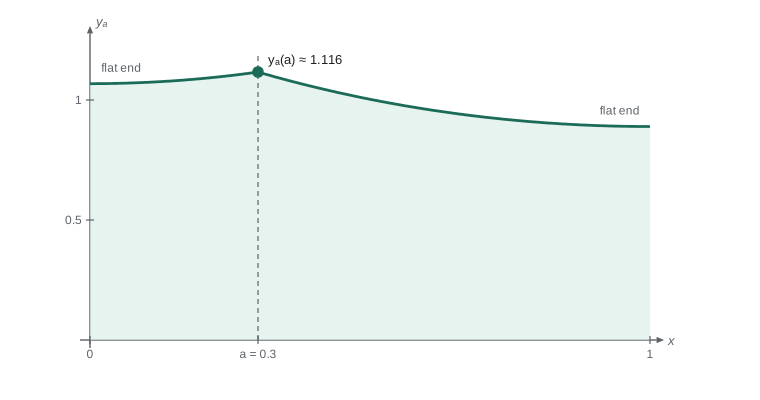
# Riesz representer of u -> u(a) in H^1(0,1), computed numerically and compared with the cosh formula.
import math

N, a = 400, 0.3
h = 1 / N
k = round(a * N)                         # grid index of the point a
# Discrete H^1 inner product <u, v> = h * sum u_i v_i (trapezoid) + sum (u_{i+1}-u_i)(v_{i+1}-v_i)/h.
# The representer y solves G y = e_k, where G is the matrix of this inner product.
w = [h] * (N + 1); w[0] = w[N] = h / 2
G = [[0.0] * (N + 1) for _ in range(N + 1)]
for i in range(N + 1):
    G[i][i] += w[i]
for i in range(N):
    G[i][i] += 1 / h; G[i + 1][i + 1] += 1 / h; G[i][i + 1] -= 1 / h; G[i + 1][i] -= 1 / h
# tridiagonal solve (Thomas algorithm)
sub = [G[i][i - 1] if i else 0.0 for i in range(N + 1)]
dia = [G[i][i] for i in range(N + 1)]
sup = [G[i][i + 1] if i < N else 0.0 for i in range(N + 1)]
rhs = [1.0 if i == k else 0.0 for i in range(N + 1)]
for i in range(1, N + 1):
    m = sub[i] / dia[i - 1]
    dia[i] -= m * sup[i - 1]; rhs[i] -= m * rhs[i - 1]
y = [0.0] * (N + 1)
y[N] = rhs[N] / dia[N]
for i in range(N - 1, -1, -1):
    y[i] = (rhs[i] - sup[i] * y[i + 1]) / dia[i]

exact = lambda x: math.cosh(min(x, a)) * math.cosh(1 - max(x, a)) / math.sinh(1)
err = max(abs(y[i] - exact(i * h)) for i in range(N + 1))
print(f"max |numerical - exact| = {err:.2e}")
print(f"y_a(a) = {y[k]:.5f} (exact {exact(a):.5f}), so the norm of point evaluation is {math.sqrt(exact(a)):.5f}")
# check the reproducing property on a test function u(x) = x^2
u = [(i * h) ** 2 for i in range(N + 1)]
ip = sum(w[i] * u[i] * y[i] for i in range(N + 1)) + sum((u[i + 1] - u[i]) * (y[i + 1] - y[i]) / h for i in range(N))
print(f"<u, y_a> for u = x^2: {ip:.6f}   u(a) = {a * a:.6f}")

max |numerical - exact| = 6.39e-07
y_a(a) = 1.11647 (exact 1.11647), so the norm of point evaluation is 1.05663
<u, y_a> for u = x^2: 0.090000   u(a) = 0.090000

The discrete problem is a finite-dimensional instance of the Riesz theorem: on \(\mathbb{R}^{N+1}\) with the inner product \(\langle u, v \rangle = u^{\mathsf{T}} G v\), the representer of the functional \(u \mapsto u_k\) is \(G^{-1} e_k\). The numbers confirm the theory: the representer converges to the cosh formula, and the reproducing property holds. Spaces in which point evaluations are bounded, so that every point has a representer, are called reproducing kernel Hilbert spaces, and the function \((x, a) \mapsto y_a(x)\) is the reproducing kernel. They are the setting of spline interpolation and of kernel methods in machine learning.

Adjoint operators

Theorem 6.2. Let \(H, K\) be Hilbert spaces and \(T \in B(H, K)\). There is a unique \(T^* \in B(K, H)\) with \(\langle Tx, y \rangle = \langle x, T^* y \rangle\) for all \(x \in H\) and \(y \in K\). Moreover \(\|T^*\| = \|T\|\), \(T^{**} = T\) and \(\|T^* T\| = \|T\|^2\).

Proof. Fix \(y \in K\). The functional \(x \mapsto \langle Tx, y \rangle\) is linear and bounded by \(\|T\| \, \|y\|\), so by Riesz there is a unique vector, which we call \(T^* y\), with \(\langle Tx, y \rangle = \langle x, T^* y \rangle\) and \(\|T^* y\| \le \|T\| \, \|y\|\). Uniqueness of representers shows \(T^*\) is linear; for example \(\langle x, T^*(y + z) \rangle = \langle Tx, y \rangle + \langle Tx, z \rangle = \langle x, T^* y + T^* z \rangle\). So \(T^* \in B(K, H)\) with \(\|T^*\| \le \|T\|\). Taking conjugates in the defining identity gives \(\langle T^* y, x \rangle = \langle y, Tx \rangle\), so \(T^{**} = T\), and then \(\|T\| = \|T^{**}\| \le \|T^*\|\). Finally \(\|T^* T\| \le \|T^*\| \, \|T\| = \|T\|^2\), and for \(\|x\| \le 1\), \(\|Tx\|^2 = \langle T^* T x, x \rangle \le \|T^* T\|\), so \(\|T\|^2 \le \|T^* T\|\). \(\blacksquare\)

The identity \(\|T^* T\| = \|T\|^2\) is called the C*-identity; an algebra of operators closed under adjoints and complete in the operator norm is a C*-algebra, the starting point of operator algebra theory. The algebraic rules \((S + T)^* = S^* + T^*\), \((\alpha T)^* = \overline{\alpha} T^*\) and \((ST)^* = T^* S^*\) follow directly from uniqueness.

Examples. (a) A matrix acting on \(\mathbb{C}^n\) has adjoint its conjugate transpose. (b) An integral operator \(Ku(x) = \int k(x, y) u(y) \, dy\) on \(L^2\) with square-integrable kernel has adjoint \(K^* v(y) = \int \overline{k(x, y)} v(x) \, dx\), the integral operator with kernel \(k^*(x, y) = \overline{k(y, x)}\); the proof is Fubini's theorem. (c) The right shift \(S\) on \(\ell^2\) has adjoint the left shift: \(\langle Sx, y \rangle = \sum_{n \ge 1} x_n \overline{y_{n+1}} = \langle x, (y_2, y_3, \ldots) \rangle\). (d) Multiplication by a bounded function \(g\) on \(L^2(\mu)\) has adjoint multiplication by \(\overline{g}\). (e) The Volterra operator \(Vu(x) = \int_0^x u\) on \(L^2(0, 1)\) has kernel \(\mathbf{1}_{y < x}\), so \(V^* v(x) = \int_x^1 v\).

Kernels and ranges

Theorem 6.3. For \(T \in B(H, K)\), \(\ker T^* = (\operatorname{ran} T)^\perp\) and \(\overline{\operatorname{ran} T} = (\ker T^*)^\perp\). Likewise \(\ker T = (\operatorname{ran} T^*)^\perp\).

Proof. \(y \in \ker T^*\) iff \(\langle x, T^* y \rangle = 0\) for all \(x\) iff \(\langle Tx, y \rangle = 0\) for all \(x\) iff \(y \perp \operatorname{ran} T\). Taking orthogonal complements and using \(M^{\perp\perp} = \overline{M}\) gives the second identity. The third is the first applied to \(T^*\). \(\blacksquare\)

This is the infinite-dimensional form of the fact that \(Ax = b\) is solvable exactly when \(b\) is orthogonal to the null space of \(A^*\). In infinite dimensions there is a catch: the theorem describes only the closure of the range. If \(y \perp \ker T^*\), then \(y\) is a limit of vectors \(Tx_n\), but the equation \(Tx = y\) may have no solution. For the Volterra operator, \(\ker V^* = \{0\}\), so the range of \(V\) is dense in \(L^2\), yet it consists only of absolutely continuous functions vanishing at \(0\) and is far from closed. Operators with closed range, such as the Fredholm operators of lesson 10, are those for which the orthogonality condition is also sufficient.

Self-adjoint, unitary and normal operators

An operator \(T \in B(H)\) is self-adjoint if \(T^* = T\), unitary if \(T^* T = T T^* = I\), and normal if \(T^* T = T T^*\). Orthogonal projections are self-adjoint (Theorem 4.6). Unitary operators are exactly the surjective isometries, since \(\langle Ux, Uy \rangle = \langle U^* U x, y \rangle\). The Fourier coefficient map of lesson 5 is unitary from \(L^2(-\pi, \pi)\) (with the normalized measure) onto \(\ell^2(\mathbb{Z})\), and Plancherel's theorem of 1910 says the Fourier transform extends to a unitary operator on \(L^2(\mathbb{R})\). The right shift is an isometry that is not unitary, and it is not normal: \(S^* S = I\) while \(S S^*\) is the projection onto the vectors with first entry zero.

Proposition 6.4. If \(T\) is self-adjoint then \(\langle Tx, x \rangle\) is real for every \(x\). On a complex Hilbert space the converse holds, and \(T = 0\) whenever \(\langle Tx, x \rangle = 0\) for all \(x\). Proof: \(\langle Tx, x \rangle = \langle x, Tx \rangle = \overline{\langle Tx, x \rangle}\). For the converse, the complex polarization identity \(4\langle Tx, y \rangle = \sum_{k=0}^{3} i^k \langle T(x + i^k y), x + i^k y \rangle\) expresses all values \(\langle Tx, y \rangle\) through the quadratic form. If the form is real, then \(\langle Tx, y \rangle = \overline{\langle Ty, x \rangle} = \langle x, Ty \rangle\), so \(T = T^*\); if it vanishes, \(\langle Tx, y \rangle = 0\) for all \(x, y\). \(\blacksquare\) The real case is different: rotation by a right angle in \(\mathbb{R}^2\) satisfies \(\langle Tx, x \rangle = 0\) for every \(x\) but is not zero.