Capstone: unbounded operators, quantum mechanics and partial differential equations

Differentiation is the most important linear operation in analysis, and lesson 1 showed that it is not bounded. The Hellinger–Toeplitz theorem of lesson 8 showed more: a symmetric operator defined on an entire Hilbert space is automatically bounded, so the symmetric differential operators of physics, momentum and energy among them, can only be defined on dense subspaces. This capstone lesson develops the language for such operators: domains, closed operators, adjoints, and the crucial distinction between symmetric and self-adjoint operators. It then applies everything in the course to two great subjects. In quantum mechanics, observables are self-adjoint operators, and we derive the energy levels of a particle in a box and the Heisenberg uncertainty principle. In partial differential equations, the Riesz representation theorem and its extension, the Lax–Milgram theorem, give weak solutions of boundary value problems, and Galerkin's method computes them. A capstone project solves one boundary value problem in three ways and checks that they agree.

Unbounded operators

Definition 12.1. An operator in a Hilbert space \(H\) is a linear map \(T : D(T) \to H\) defined on a subspace \(D(T)\), its domain. It is densely defined if \(D(T)\) is dense, and closed if its graph \(\{(x, Tx) : x \in D(T)\}\) is closed in \(H \times H\). An operator \(S\) extends \(T\), written \(T \subseteq S\), if \(D(T) \subseteq D(S)\) and \(S = T\) on \(D(T)\).

The domain is part of the operator: the same formula on different domains gives different operators with different properties. By the closed graph theorem, a closed operator defined on all of \(H\) is bounded, so the interesting closed operators have proper dense domains. The natural domains for differential operators are Sobolev spaces. On \((0, 1)\), \(H^1(0, 1)\) is the space of \(u \in L^2\) of the form \(u(x) = c + \int_0^x g\) with \(g \in L^2\), with \(u^{\prime} = g\); its elements are continuous, so boundary values make sense. Likewise \(H^2(0, 1)\) consists of \(u \in H^1\) with \(u^{\prime} \in H^1\).

Definition 12.2. Let \(T\) be densely defined. Its adjoint \(T^*\) has domain \(D(T^*)\), the set of \(y \in H\) for which \(x \mapsto \langle Tx, y \rangle\) is bounded on \(D(T)\), and for such \(y\), \(T^*y\) is the unique vector with \(\langle Tx, y \rangle = \langle x, T^* y \rangle\) for all \(x \in D(T)\). Uniqueness uses density of \(D(T)\), and existence uses the Riesz theorem applied to the continuous extension of the functional to \(H\). The operator \(T\) is symmetric if \(\langle Tx, y \rangle = \langle x, Ty \rangle\) for all \(x, y \in D(T)\), that is, \(T \subseteq T^*\), and self-adjoint if \(T = T^*\), domains included.

The adjoint of a densely defined operator is always closed. A symmetric operator is closable, and a self-adjoint operator is closed and maximal among symmetric operators: it has no proper symmetric extension. The difference between symmetric and self-adjoint is invisible for bounded operators and decisive for unbounded ones, because only self-adjoint operators have a spectral theorem, real spectrum and a well-defined exponential \(e^{-itT}\).

Momentum on an interval

Let \(P = -i \frac{d}{dx}\) on \(L^2(0, 1)\). For \(u, v \in H^1(0, 1)\), integration by parts gives \[\langle Pu, v \rangle - \langle u, Pv \rangle = -i \int_0^1 (u^{\prime} \overline{v} + u \overline{v^{\prime}}) = -i \big(u(1)\overline{v(1)} - u(0)\overline{v(0)}\big).\] The boundary term decides everything. (a) On \(D(P_0) = \{u \in H^1 : u(0) = u(1) = 0\}\), the boundary term vanishes, so \(P_0\) is symmetric. But \(P_0^*\) is \(-i\frac{d}{dx}\) on all of \(H^1\): for \(v \in H^1\) the boundary term vanishes as long as \(u\) vanishes at both ends. So \(D(P_0) \subsetneq D(P_0^*)\), and \(P_0\) is symmetric but not self-adjoint. It has no eigenvalues at all, since \(-iu^{\prime} = \lambda u\) with \(u(0) = 0\) forces \(u = 0\). (b) For \(\theta \in [0, 2\pi)\), let \(D(P_\theta) = \{u \in H^1 : u(1) = e^{i\theta} u(0)\}\). For \(u, v\) in this domain the boundary term is \(-i u(0)\overline{v(0)}(|e^{i\theta}|^2 - 1) = 0\), so \(P_\theta\) is symmetric, and a short argument shows \(D(P_\theta^*) = D(P_\theta)\): \(P_\theta\) is self-adjoint. Its eigenfunctions are \(e^{i(2\pi n + \theta)x}\) with eigenvalues \(2\pi n + \theta\), \(n \in \mathbb{Z}\), and they form an orthonormal basis of \(L^2(0, 1)\), a shifted Fourier basis.

So the symmetric operator \(P_0\) has a whole circle of self-adjoint extensions \(P_\theta\), with different spectra. John von Neumann's theory of deficiency indices, developed in 1929 and 1930, classifies the self-adjoint extensions of any closed symmetric operator; Hermann Weyl had found the analogous phenomenon for second-order differential operators in 1910 in his limit-point and limit-circle theory. Physically, choosing an extension means choosing boundary conditions, and different choices describe different physical systems: \(\theta\) is the phase picked up by a particle moving on a ring threaded by a magnetic flux, the Aharonov–Bohm effect.

The spectral theorem and Stone's theorem

Von Neumann proved in 1929 that every self-adjoint operator, bounded or not, has a spectral resolution: there is a projection-valued measure \(E\) on the Borel sets of \(\mathbb{R}\) with \(T = \int \lambda \, dE(\lambda)\). Equivalently, \(T\) is unitarily equivalent to multiplication by a real function on some \(L^2(\mu)\). When \(T\) has a compact inverse, as for the Dirichlet Laplacian below, the resolution is a sum over an orthonormal basis of eigenvectors, exactly as in lesson 11. Marshall Stone proved in 1932 that self-adjoint operators correspond exactly to strongly continuous one-parameter unitary groups: for self-adjoint \(H\), \(U(t) = e^{-itH}\) is unitary, \(U(s + t) = U(s)U(t)\), \(U(t)x \to x\) as \(t \to 0\), and \(\frac{d}{dt} U(t)x = -iHU(t)x\) for \(x \in D(H)\); conversely every such group arises this way from a unique self-adjoint generator. This is why self-adjointness, not mere symmetry, is required of a quantum Hamiltonian: it is exactly the condition for the Schrödinger equation \(i\frac{d\psi}{dt} = H\psi\) to have a unitary, probability-preserving solution for all time.

The Dirichlet Laplacian and the particle in a box

Let \(A = -\frac{d^2}{dx^2}\) with \(D(A) = \{u \in H^2(0, 1) : u(0) = u(1) = 0\}\). Lesson 11 showed that \(A\) is the inverse of the Green's operator \(G\): for \(f \in L^2\), \(u = Gf\) is the unique element of \(D(A)\) with \(Au = f\). If \(B\) is a bounded, injective, self-adjoint operator, then \(B^{-1}\), with domain the range of \(B\), is self-adjoint, because the graph of \(B^{-1}\) is the graph of \(B\) with its two coordinates exchanged, and taking adjoints commutes with this exchange. Hence \(A = G^{-1}\) is self-adjoint, and the eigenbasis of \(G\) diagonalizes it: \(A\phi_n = n^2\pi^2 \phi_n\) with \(\phi_n = \sqrt{2}\sin n\pi x\), and \(D(A) = \{u : \sum n^4\pi^4 |\langle u, \phi_n \rangle|^2 < \infty\}\).

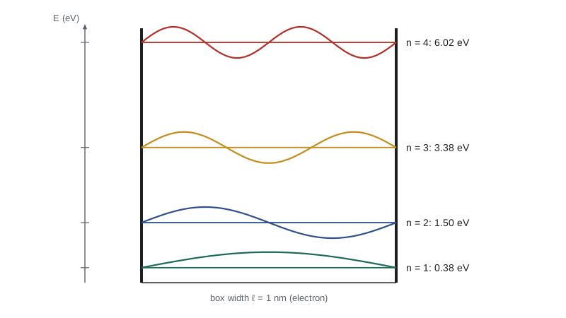
In quantum mechanics a particle of mass \(m\) confined to an interval of length \(\ell\) has state space \(L^2(0, \ell)\) and Hamiltonian \(H = -\frac{\hbar^2}{2m} \frac{d^2}{dx^2}\) with Dirichlet boundary conditions, by rescaling the operator \(A\). The states are unit vectors \(\psi\), and the expected value of an observable \(B\) in the state \(\psi\) is \(\langle B\psi, \psi \rangle\). The possible energies are the eigenvalues \[E_n = \frac{n^2 \pi^2 \hbar^2}{2 m \ell^2}, \qquad n = 1, 2, 3, \ldots,\] with stationary states \(\sqrt{2/\ell}\sin(n\pi x / \ell)\), and a general state evolves as \(\psi(t) = \sum_n e^{-iE_n t/\hbar} \langle \psi(0), \phi_n \rangle \phi_n\). The energy is quantized because \(H\) has a compact inverse, a purely functional-analytic fact.

The uncertainty principle

Theorem 12.3 (Robertson, 1929). Let \(A, B\) be symmetric operators and \(\psi\) a unit vector in \(D(AB) \cap D(BA)\). Write \(\langle A \rangle = \langle A\psi, \psi \rangle\) and \(\Delta A = \|(A - \langle A \rangle)\psi\|\), the standard deviation of \(A\) in the state \(\psi\). Then \[\Delta A \, \Delta B \ge \frac{1}{2} \big| \langle (AB - BA)\psi, \psi \rangle \big|.\]

Proof. Let \(A_0 = A - \langle A \rangle\) and \(B_0 = B - \langle B \rangle\), which are symmetric with \(A_0 B_0 - B_0 A_0 = AB - BA\) on the relevant domain. By symmetry, \(\langle (A_0 B_0 - B_0 A_0)\psi, \psi \rangle = \langle B_0\psi, A_0\psi \rangle - \langle A_0\psi, B_0\psi \rangle = -2i \operatorname{Im} \langle A_0\psi, B_0\psi \rangle\). By Cauchy–Schwarz, \(|\operatorname{Im}\langle A_0\psi, B_0\psi \rangle| \le \|A_0\psi\| \, \|B_0\psi\| = \Delta A \, \Delta B\). \(\blacksquare\)

For position \(X\psi(x) = x\psi(x)\) and momentum \(P = -i\hbar\frac{d}{dx}\) on \(L^2(\mathbb{R})\), the product rule gives \((XP - PX)\psi = i\hbar\psi\) for smooth rapidly decaying \(\psi\), so \(\Delta X \, \Delta P \ge \frac{\hbar}{2}\): this is Heisenberg's uncertainty relation of 1927, as a theorem about the Cauchy–Schwarz inequality. Equality holds for Gaussian wave packets. The canonical commutation relation \(XP - PX = i\hbar I\) also explains why \(X\) and \(P\) must be unbounded. Theorem 12.4 (Wintner 1947, Wielandt 1949). There are no bounded operators with \(AB - BA = I\). Proof: induction gives \(AB^n - B^nA = nB^{n-1}\) for \(n \ge 1\). If some \(B^{k} = 0\) with \(k\) minimal, then \(kB^{k-1} = AB^k - B^kA = 0\), contradicting minimality (for \(k = 1\) it reads \(I = 0\)). So \(B^{n-1} \ne 0\) for all \(n\), and \(n\|B^{n-1}\| \le 2\|A\| \, \|B\| \, \|B^{n-1}\|\) gives \(n \le 2\|A\| \, \|B\|\) for every \(n\), which is absurd. \(\blacksquare\) In finite dimensions the trace gives a quicker proof, since \(\operatorname{tr}(AB - BA) = 0 \ne \operatorname{tr} I\).

Weak solutions of boundary value problems

Consider \(-u^{\prime\prime} = f\) on \((0, 1)\) with \(u(0) = u(1) = 0\) and \(f \in L^2\). Multiplying by a test function \(v\) that vanishes at the ends and integrating by parts gives the weak formulation: find \(u \in H^1_0(0, 1) = \{u \in H^1 : u(0) = u(1) = 0\}\) with \[\int_0^1 u^{\prime} \, \overline{v^{\prime}} = \int_0^1 f \, \overline{v} \quad \text{for all } v \in H^1_0(0, 1).\] Every classical solution is a weak solution, and the weak problem makes sense for much rougher data, in any dimension: for \(-\Delta u = f\) in a bounded domain \(\Omega \subseteq \mathbb{R}^n\) it reads \(\int_\Omega \nabla u \cdot \overline{\nabla v} = \int_\Omega f\overline{v}\).

Lemma 12.5 (Poincaré inequality). For \(u \in H^1_0(0, 1)\), \(\|u\|_2 \le \frac{1}{\sqrt{2}} \|u^{\prime}\|_2\). Proof: \(u(x) = \int_0^x u^{\prime}\), so by Cauchy–Schwarz \(|u(x)|^2 \le x \int_0^1 |u^{\prime}|^2\), and integrating over \(x\) gives \(\|u\|_2^2 \le \frac{1}{2}\|u^{\prime}\|_2^2\). \(\blacksquare\) The best constant is \(\frac{1}{\pi}\), the square root of the largest eigenvalue of the Green's operator, by the variational characterization of lesson 11. Consequently \(\langle u, v \rangle_a = \int u^{\prime}\overline{v^{\prime}}\) is an inner product on \(H^1_0\) whose norm is equivalent to the \(H^1\) norm, and \(H^1_0\) is complete in it, being a closed subspace of \(H^1\) (point evaluations are continuous by lesson 6).

Theorem 12.6. For every \(f \in L^2(0, 1)\) the weak problem has a unique solution \(u \in H^1_0\), and \(\|u^{\prime}\|_2 \le \frac{1}{\sqrt{2}} \|f\|_2\). Proof: the functional \(F(v) = \int_0^1 v \overline{f}\) satisfies \(|F(v)| \le \|f\|_2 \|v\|_2 \le \frac{1}{\sqrt{2}}\|f\|_2 \|v^{\prime}\|_2\), so it is bounded on \((H^1_0, \langle \cdot, \cdot \rangle_a)\). By the Riesz theorem there is a unique \(u\) with \(\langle v, u \rangle_a = F(v)\) for all \(v\); conjugating gives the weak formulation, and \(\|u\|_a = \|F\|\) gives the estimate. \(\blacksquare\) This is Hilbert's rescue of Dirichlet's principle in modern form: the weak solution minimizes the energy \(\frac{1}{2}\int|v^{\prime}|^2 - \operatorname{Re}\int f\overline{v}\), and the Hilbert space makes the minimizer exist.

Theorem 12.7 (Lax and Milgram, 1954). Let \(a\) be a sesquilinear form on a Hilbert space \(V\), bounded, \(|a(u, v)| \le M\|u\|\|v\|\), and coercive, \(\operatorname{Re} a(u, u) \ge \alpha \|u\|^2\) with \(\alpha > 0\). Then for every \(F \in V^*\) there is a unique \(u \in V\) with \(a(v, u) = F(v)\) for all \(v \in V\), and \(\|u\| \le \frac{1}{\alpha}\|F\|\). (The order \(a(v, u)\) matches our convention that forms are linear in the first variable.)

Proof. For fixed \(u\), \(v \mapsto a(v, u)\) is a bounded linear functional, so by Riesz it equals \(\langle v, Au \rangle\) for a unique \(Au \in V\). The map \(A\) is linear and bounded with \(\|A\| \le M\). Coercivity gives \(\alpha\|u\|^2 \le \operatorname{Re} a(u, u) = \operatorname{Re}\langle u, Au \rangle \le \|u\| \, \|Au\|\), so \(\|Au\| \ge \alpha\|u\|\). Hence \(A\) is injective with closed range. Its range is dense: if \(w \perp \operatorname{ran} A\), then \(\alpha\|w\|^2 \le \operatorname{Re}\langle w, Aw \rangle = 0\). So \(A\) is bijective. Writing \(F(v) = \langle v, y \rangle\) by Riesz, the equation \(a(v, u) = F(v)\) for all \(v\) becomes \(Au = y\), with the unique solution \(u = A^{-1}y\) and \(\|u\| \le \frac{1}{\alpha}\|y\| = \frac{1}{\alpha}\|F\|\). \(\blacksquare\)

Peter Lax and Arthur Milgram proved the theorem in 1954 to handle equations such as \(-u^{\prime\prime} + bu^{\prime} + cu = f\) whose forms are not symmetric, so that the Riesz theorem does not apply directly. Galerkin's method computes the solution: choose a finite-dimensional subspace \(V_h \subseteq V\), for instance the continuous piecewise linear functions on a mesh of width \(h\), and find \(u_h \in V_h\) with \(a(v, u_h) = F(v)\) for all \(v \in V_h\), a finite linear system. Subtracting the two equations gives Galerkin orthogonality \(a(v, u - u_h) = 0\) for \(v \in V_h\), and then for any \(v_h \in V_h\), \(\alpha\|u - u_h\|^2 \le |a(u - u_h, u - u_h)| = |a(u - v_h, u - u_h)| \le M\|u - v_h\|\|u - u_h\|\). This is Céa's lemma of 1964: \(\|u - u_h\| \le \frac{M}{\alpha}\inf_{v_h \in V_h}\|u - v_h\|\), so the computed solution is as good as the best approximation from \(V_h\), up to a constant. With piecewise linear elements this is the finite element method, whose mathematical origins go back to Richard Courant in 1943 and whose engineering use took off in the 1950s and 1960s.

Capstone project: one problem, three solutions

Solve \(-u^{\prime\prime} = 1\) on \((0, 1)\) with \(u(0) = u(1) = 0\) in three ways. (1) Directly: \(u(x) = \frac{1}{2}x(1 - x)\). (2) By the spectral theorem: with \(\phi_n = \sqrt{2}\sin n\pi x\), \(\langle 1, \phi_n \rangle = \frac{\sqrt{2}(1 - (-1)^n)}{n\pi}\), so \(u = Gf = \sum_n \frac{\langle 1, \phi_n \rangle}{n^2\pi^2}\phi_n = \sum_{n \text{ odd}} \frac{4\sin n\pi x}{n^3\pi^3}\). (3) By finite elements: with hat functions on a uniform mesh of \(N\) intervals, the Galerkin system is the tridiagonal matrix \(\frac{1}{h}(2, -1)\) times the nodal values, equal to the load vector \(h(1, \ldots, 1)\). Theory predicts that (2) converges uniformly with error of order \(n^{-2}\) after \(n\) terms, that (3) has energy-norm error of order \(h\) by Céa's lemma, and, a special feature of one dimension, that (3) is exact at the nodes.

# Capstone: -u'' = 1 on (0,1), u(0) = u(1) = 0, solved exactly, by eigenfunctions, and by finite elements.
import math

exact = lambda x: x * (1 - x) / 2

def series(x, terms):
    return sum(4 * math.sin(n * math.pi * x) / (n * math.pi) ** 3 for n in range(1, 2 * terms, 2))

xs = [k / 200 for k in range(201)]
for terms in (1, 3, 10, 30):
    err = max(abs(series(x, terms) - exact(x)) for x in xs)
    print(f"eigenfunction series, {terms:2d} odd terms: max error = {err:.2e}")

def fem(N):
    h = 1 / N
    n = N - 1                                   # interior nodes
    a, b = [2 / h] * n, [-1 / h] * n            # tridiagonal stiffness matrix
    rhs = [h] * n
    for i in range(1, n):                       # Thomas algorithm
        m = b[i] / a[i - 1]
        a[i] -= m * b[i - 1]; rhs[i] -= m * rhs[i - 1]
    u = [0.0] * n
    u[-1] = rhs[-1] / a[-1]
    for i in range(n - 2, -1, -1):
        u[i] = (rhs[i] - b[i] * u[i + 1]) / a[i]
    nodes = [0.0] + u + [0.0]
    nodal_err = max(abs(nodes[k] - exact(k * h)) for k in range(N + 1))
    # energy norm of the error: on each element u_h' is constant, u' = 1/2 - x
    e2 = 0.0
    for k in range(N):
        slope = (nodes[k + 1] - nodes[k]) / h
        x0, x1 = k * h, (k + 1) * h
        # integral of (1/2 - x - slope)^2 over [x0, x1], exact for a quadratic
        f = lambda x: (0.5 - x - slope) ** 2
        e2 += (x1 - x0) / 6 * (f(x0) + 4 * f((x0 + x1) / 2) + f(x1))
    return nodal_err, math.sqrt(e2)

for N in (4, 8, 16, 32):
    ne, ee = fem(N)
    print(f"finite elements, N = {N:2d}: max nodal error = {ne:.1e}, energy-norm error = {ee:.5f}  (h / sqrt(12) = {1 / N / math.sqrt(12):.5f})")

# particle in a box: electron in a 1 nm box, energies in electronvolts
hbar, me, eV, L = 1.054571817e-34, 9.1093837015e-31, 1.602176634e-19, 1e-9
for n in range(1, 5):
    print(f"E_{n} = {(n * math.pi * hbar) ** 2 / (2 * me * L ** 2) / eV:.3f} eV")

eigenfunction series,  1 odd terms: max error = 5.32e-03
eigenfunction series,  3 odd terms: max error = 6.74e-04
eigenfunction series, 10 odd terms: max error = 6.15e-05
eigenfunction series, 30 odd terms: max error = 6.85e-06
finite elements, N =  4: max nodal error = 1.4e-17, energy-norm error = 0.07217  (h / sqrt(12) = 0.07217)
finite elements, N =  8: max nodal error = 1.4e-17, energy-norm error = 0.03608  (h / sqrt(12) = 0.03608)
finite elements, N = 16: max nodal error = 1.4e-17, energy-norm error = 0.01804  (h / sqrt(12) = 0.01804)
finite elements, N = 32: max nodal error = 3.9e-16, energy-norm error = 0.00902  (h / sqrt(12) = 0.00902)
E_1 = 0.376 eV
E_2 = 1.504 eV
E_3 = 3.384 eV
E_4 = 6.016 eV

The results confirm each prediction. The series error falls by roughly a factor of nine when the number of terms triples, consistent with order \(n^{-2}\). The finite element nodal values agree with the exact solution to rounding error, and the energy-norm error is exactly \(\frac{h}{\sqrt{12}}\), halving with each halving of \(h\): on each element the error derivative is a linear function of mean zero and range \(h\). The particle-in-a-box energies, \(0.376\) electronvolts for the ground state of an electron confined to a box \(1\) nm wide, set the scale for quantum dots, semiconductor crystals a few nm across whose emission wavelengths are tuned by their size.