Why functional analysis: linear algebra in infinite dimensions

Linear algebra studies vector spaces of finite dimension: \(\mathbb{R}^n\), \(\mathbb{C}^n\), spaces of matrices and polynomials of bounded degree. Its central results, such as the rank–nullity theorem, the existence of eigenvalues for complex matrices and the spectral theorem for symmetric matrices, make finite-dimensional problems almost completely solvable. Analysis constantly produces vector spaces that are not finite dimensional: the continuous functions on an interval, the square-integrable functions of MATH-441, the solutions of a differential equation with a forcing term, the sequences of Fourier coefficients of a signal. Functional analysis is the study of such spaces together with a notion of distance or size, and of the linear maps between them. Its theorems tell us which parts of linear algebra survive in infinite dimensions, which parts fail, and what replaces them.

This first lesson sets the scene. We recall what a norm is, look at the three most important norms on \(\mathbb{R}^n\), prove that all norms on a finite-dimensional space are equivalent, and then see five ways in which infinite-dimensional spaces behave differently. Each failure motivates one of the main theorems of the course. We close with the historical problem that started the subject, the integral equation of Fredholm, and a road map of the twelve lessons.

Norms

Definition 1.1. Let \(X\) be a vector space over \(\mathbb{K} = \mathbb{R}\) or \(\mathbb{C}\). A norm on \(X\) is a function \(\|\cdot\| : X \to [0, \infty)\) such that for all \(x, y \in X\) and \(\alpha \in \mathbb{K}\): (N1) \(\|x\| = 0\) only when \(x = 0\); (N2) \(\|\alpha x\| = |\alpha| \, \|x\|\); (N3) \(\|x + y\| \le \|x\| + \|y\|\). The pair \((X, \|\cdot\|)\) is a normed space. A function satisfying (N2) and (N3) but perhaps not (N1) is a seminorm.

Every norm defines a metric \(d(x, y) = \|x - y\|\), so the language of MATH-341 applies: open and closed balls, convergent and Cauchy sequences, continuity, compactness and completeness. The metric of a norm has two extra properties that a general metric lacks. It is translation invariant, \(d(x + z, y + z) = d(x, y)\), and it scales, \(d(\alpha x, \alpha y) = |\alpha| d(x, y)\). Consequently the whole geometry of a normed space is encoded in its closed unit ball \(B_X = \{x : \|x\| \le 1\}\): every other ball is a translate of a dilate of it. A reverse triangle inequality also holds, \(\big| \|x\| - \|y\| \big| \le \|x - y\|\), so the norm itself is a continuous, indeed 1-Lipschitz, function on \(X\).

On \(\mathbb{K}^n\) the three standard norms are \[\|x\|_1 = \sum_{i=1}^{n} |x_i|, \qquad \|x\|_2 = \Big(\sum_{i=1}^{n} |x_i|^2\Big)^{1/2}, \qquad \|x\|_\infty = \max_{1 \le i \le n} |x_i|.\] More generally \(\|x\|_p = \big(\sum |x_i|^p\big)^{1/p}\) for \(1 \le p < \infty\). Properties (N1) and (N2) are clear, and (N3) is Minkowski's inequality, which MATH-441 proved for \(L^p\) spaces of any measure; counting measure on \(\{1, \ldots, n\}\) gives the finite case. For \(0 < p < 1\) the formula fails (N3): with \(x = (1, 0)\) and \(y = (0, 1)\), \(\|x + y\|_p = 2^{1/p} > 2 = \|x\|_p + \|y\|_p\).

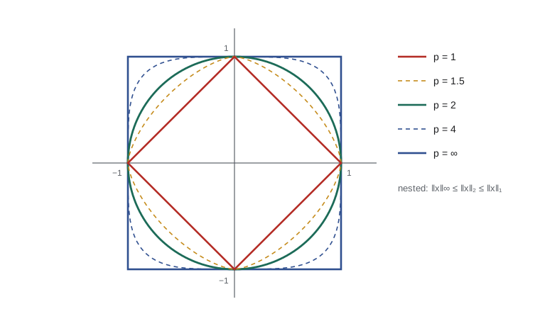
The picture already shows a fact we will prove in general: the balls are nested, \(\|x\|_\infty \le \|x\|_2 \le \|x\|_1\), and each ball contains a scaled copy of every other. Indeed \(\|x\|_1 \le n \|x\|_\infty\) and \(\|x\|_2 \le \sqrt{n} \|x\|_\infty\). The constants depend on \(n\), and this dependence is the first hint of trouble in infinite dimensions.

All norms on a finite-dimensional space are equivalent

Definition 1.2. Two norms \(\|\cdot\|_a\) and \(\|\cdot\|_b\) on \(X\) are equivalent if there are constants \(0 < c \le C\) with \(c \|x\|_a \le \|x\|_b \le C \|x\|_a\) for all \(x \in X\). Equivalent norms have the same convergent sequences, the same Cauchy sequences, the same open sets and the same compact sets.

Theorem 1.3. On a finite-dimensional vector space all norms are equivalent.

Proof. Choose a basis \(e_1, \ldots, e_n\) and identify \(X\) with \(\mathbb{K}^n\) through \(x = \sum x_i e_i\). It suffices to show that an arbitrary norm \(\|\cdot\|\) is equivalent to the Euclidean norm \(|x| = \|x\|_2\), since equivalence is transitive. By the triangle inequality and the Cauchy–Schwarz inequality in \(\mathbb{K}^n\), \[\|x\| \le \sum_{i=1}^{n} |x_i| \, \|e_i\| \le \Big(\sum_{i=1}^{n} \|e_i\|^2\Big)^{1/2} |x| = C |x|.\] Hence \(\big| \|x\| - \|y\| \big| \le \|x - y\| \le C |x - y|\), so \(\|\cdot\|\) is continuous with respect to the Euclidean metric. The Euclidean unit sphere \(S = \{x : |x| = 1\}\) is closed and bounded in \(\mathbb{K}^n\), hence compact by the Heine–Borel theorem, so the continuous function \(\|\cdot\|\) attains a minimum \(c\) on \(S\) at some point \(x_0\). Since \(x_0 \ne 0\), (N1) gives \(c = \|x_0\| > 0\). For any \(x \ne 0\), the vector \(x / |x|\) lies in \(S\), so \(\|x / |x|\| \ge c\), that is, \(\|x\| \ge c|x|\). \(\blacksquare\)

The proof uses compactness of the unit sphere in an essential way, and that is precisely what fails in infinite dimensions. Three corollaries follow at once. Every finite-dimensional normed space is complete, since Cauchy sequences in any norm are Cauchy in the Euclidean norm. Every finite-dimensional subspace of a normed space is closed, since it is complete. Every closed and bounded subset of a finite-dimensional normed space is compact. Finally, every linear map from a finite-dimensional normed space to any normed space is continuous: with the notation of the proof, \(\|Tx\| \le \sum |x_i| \|Te_i\| \le C' |x| \le (C'/c) \|x\|\).

Five things that go wrong

Failure 1: norms need not be equivalent. On the space \(C[0, 1]\) of continuous functions consider the supremum norm \(\|f\|_\infty = \max |f|\) and the integral norm \(\|f\|_1 = \int_0^1 |f|\). Always \(\|f\|_1 \le \|f\|_\infty\), but no reverse inequality holds: the tent function \(f_n\) of height \(1\) supported on \([0, \frac{1}{n}]\) has \(\|f_n\|_\infty = 1\) and \(\|f_n\|_1 = \frac{1}{2n}\). So \(f_n \to 0\) in one norm and not in the other. Lesson 2 shows that \(C[0, 1]\) is complete in the first norm and not in the second, so the choice of norm is a real decision with consequences.

Failure 2: closed bounded sets need not be compact. In the space \(\ell^2\) of square-summable sequences, let \(e_n\) be the sequence with \(1\) in position \(n\) and \(0\) elsewhere. Every \(e_n\) lies in the closed unit ball, and \(\|e_n - e_m\|_2 = \sqrt{2}\) for \(n \ne m\), so no subsequence is Cauchy and the unit ball is not compact. Lesson 2 proves Riesz's lemma, which shows this happens in every infinite-dimensional normed space. Much of functional analysis consists of finding substitutes for compactness: compact operators in lessons 10 and 11, and weak compactness in lesson 9.

Failure 3: linear maps need not be continuous. Let \(P\) be the space of polynomials on \([0, 1]\) with the supremum norm, and let \(D p = p'\). The monomials \(p_n(x) = x^n\) have \(\|p_n\|_\infty = 1\), while \(\|D p_n\|_\infty = \|n x^{n-1}\|_\infty = n\). So \(D\) maps the unit ball onto an unbounded set, and \(p_n / n \to 0\) while \(D(p_n / n) = x^{n-1}\) does not tend to zero. Differentiation, one of the most important linear operations in analysis, is not continuous in the natural norm. Lesson 3 develops the theory of bounded operators, and lesson 12 returns to unbounded ones such as \(D\), which are central to quantum mechanics.

Failure 4: injective does not imply surjective. On \(\ell^2\) define the right shift \(S(x_1, x_2, \ldots) = (0, x_1, x_2, \ldots)\). It preserves norms, so it is injective, but its range consists of sequences with first entry zero and misses \(e_1\). In finite dimensions rank–nullity forbids this. The left shift \(S^*(x_1, x_2, \ldots) = (x_2, x_3, \ldots)\) is surjective but kills \(e_1\). These two operators reappear throughout the course; lesson 10 measures their failure with the Fredholm index.

Failure 5: algebraic bases are useless. Every vector space has a Hamel basis, a set \(B\) such that every vector is a unique finite linear combination of elements of \(B\), but the proof uses Zorn's lemma and gives no description. Lesson 8 shows that a Hamel basis of an infinite-dimensional complete normed space must be uncountable. What analysis needs instead are bases that allow infinite sums, such as the orthonormal bases of lesson 5, where every \(x\) in a Hilbert space is \(\sum_k \langle x, e_k \rangle e_k\), with convergence in norm.

# Finite versus infinite dimensions: norm comparisons and the failure of compactness.
import math

def norm(x, p):
    if p == math.inf:
        return max(abs(t) for t in x)
    return sum(abs(t) ** p for t in x) ** (1 / p)

# In R^n the worst ratio between the 1-norm and the sup-norm is n, attained at (1, ..., 1).
for n in (2, 10, 100, 1000):
    ones = [1.0] * n
    print(f"n = {n:4d}: |x|_1 / |x|_inf = {norm(ones, 1) / norm(ones, math.inf):7.1f},"
          f"  |x|_2 / |x|_inf = {norm(ones, 2) / norm(ones, math.inf):6.2f}")

# Unit vectors e_n in l^2 (truncated to length N) stay a fixed distance apart.
N = 6
e = [[1.0 if i == k else 0.0 for i in range(N)] for k in range(N)]
dists = {round(norm([a - b for a, b in zip(e[i], e[j])], 2), 6) for i in range(N) for j in range(N) if i != j}
print("distances between distinct e_n:", dists, "= sqrt(2) =", round(math.sqrt(2), 6))

# Differentiation on polynomials: sup norm of x^n on [0, 1] is 1, of its derivative n.
grid = [i / 2000 for i in range(2001)]
for n in (1, 5, 25, 125):
    p = max(abs(x ** n) for x in grid)
    dp = max(abs(n * x ** (n - 1)) for x in grid)
    print(f"n = {n:3d}: |x^n| = {p:.3f}, |D x^n| = {dp:.1f}")

n =    2: |x|_1 / |x|_inf =     2.0,  |x|_2 / |x|_inf =   1.41
n =   10: |x|_1 / |x|_inf =    10.0,  |x|_2 / |x|_inf =   3.16
n =  100: |x|_1 / |x|_inf =   100.0,  |x|_2 / |x|_inf =  10.00
n = 1000: |x|_1 / |x|_inf =  1000.0,  |x|_2 / |x|_inf =  31.62
distances between distinct e_n: {1.414214} = sqrt(2) = 1.414214
n =   1: |x^n| = 1.000, |D x^n| = 1.0
n =   5: |x^n| = 1.000, |D x^n| = 5.0
n =  25: |x^n| = 1.000, |D x^n| = 25.0
n = 125: |x^n| = 1.000, |D x^n| = 125.0

The first part of the output shows the constant \(n\) in \(\|x\|_1 \le n \|x\|_\infty\) is sharp, so there is no uniform constant once \(n\) is allowed to grow. The second part confirms the computation in failure 2, and the third confirms failure 3.

The problem that started it all: integral equations

Around 1900 the Swedish mathematician Ivar Fredholm studied equations of the form \[u(x) - \lambda \int_0^1 K(x, y) \, u(y) \, dy = f(x), \qquad 0 \le x \le 1,\] where the kernel \(K\) and the right side \(f\) are given continuous functions and \(u\) is unknown. Such equations arise when a boundary value problem for a differential equation is inverted: lesson 11 shows, for example, that \(-u'' = g\) with \(u(0) = u(1) = 0\) is equivalent to \(u(x) = \int_0^1 G(x, y) g(y) \, dy\) with \(G(x, y) = \min(x, y) - xy\). Fredholm's idea, published in a note of 1900 and a long paper in Acta Mathematica in 1903, was to replace the integral by a Riemann sum with \(n\) points, solve the resulting \(n \times n\) linear system by determinants, and let \(n \to \infty\). He found that the limiting equation behaves like a finite linear system: either it has a unique solution for every \(f\), or the homogeneous equation has nonzero solutions, and then the inhomogeneous one is solvable only for \(f\) satisfying finitely many conditions.

This dichotomy, the Fredholm alternative, is the subject of lesson 10. David Hilbert took up Fredholm's work in a series of papers from 1904 to 1910, collected in a book in 1912, and introduced the space of square-summable sequences as the natural setting for symmetric kernels. Erhard Schmidt in 1907 developed the geometry of that space, with inner products, orthogonality and projections, in language close to ours. Frigyes Riesz and Ernst Fischer proved in 1907 that \(L^2\) is complete and isomorphic to \(\ell^2\), and Maurice Fréchet introduced abstract metric spaces in his 1906 thesis. Riesz developed the \(L^p\) spaces in 1910 and the theory of compact operators in 1918. The decisive step to general normed spaces came with Stefan Banach, whose thesis was published in 1922 and whose book Théorie des opérations linéaires of 1932 fixed the subject. In the same years John von Neumann axiomatized Hilbert space, between 1927 and 1929, and used it for the mathematical foundations of quantum mechanics in a book of 1932.

Road map

Lessons 2 and 3 set up the basic objects: complete normed spaces, called Banach spaces, and the bounded linear operators between them, including the dual space of continuous linear functionals. Lessons 4 to 6 treat Hilbert spaces, where an inner product gives angles and orthogonality: the projection theorem, orthonormal bases with Fourier series as the leading example, the Riesz representation theorem and adjoint operators. Lessons 7 to 9 prove the four pillars of the general theory, the Hahn–Banach theorem, the uniform boundedness principle, the open mapping theorem and the closed graph theorem, and use them to study weak convergence and reflexivity. Lessons 10 and 11 return to Fredholm's problem with compact operators, the Fredholm alternative and the spectral theorem for compact self-adjoint operators. The capstone, lesson 12, steps beyond bounded operators to the unbounded self-adjoint operators of quantum mechanics and the weak formulation of partial differential equations.

Throughout, the guiding question is the same: which statements of finite-dimensional linear algebra remain true, under which extra hypotheses? Often the extra hypothesis is completeness, which makes the Baire category theorem available. Sometimes it is an inner product, which gives orthogonal projections. And sometimes it is compactness of an operator, which makes an infinite-dimensional problem behave like a finite one up to a small error.