Statistics and control charts for safety data

Six months into the new framework, the Dartmouth site had a bad month: four recordable injuries in about 20,000 hours, a monthly rate of 40 per 200,000 hours. The site manager, Grace Whitfield, was called to explain it at the executive meeting. Two months later the same site had a month with no injuries, and someone suggested it should be recognized. Elena asked Nina to help the leadership team answer a question they had never asked: how much of what they were reacting to was chance?

This lesson introduces the statistical tools Harrowgate Foods Ltd. uses to separate real change from noise: the Poisson model for injury counts, confidence intervals for rates, and control charts. The mathematics is light, and the scripts do the arithmetic. What matters is knowing when a change in a number is evidence and when it is not.

Injuries as random events

When many people each face a small chance of injury over many hours, the number of injuries in a period follows a pattern called the Poisson distribution, closely enough for practical purposes. The Poisson distribution has one property that explains most of the noise in safety data: its variance equals its mean. If a site expects 9 injuries a year, the standard deviation of the count is about \(\sqrt{9} = 3\), so counts from about 3 to 15 are entirely ordinary. If a site expects 2, counts from 0 to 5 are ordinary.

This means that the smaller the expected count, the larger the relative noise. A site that expects 100 injuries a year would rarely see fewer than 80 or more than 120, a swing of about 20 percent. A site that expects 4 could easily see 1 or 8, a swing of 75 percent or more. Most of Harrowgate Foods Ltd.'s sites, departments and months fall in the second group.

Confidence intervals for rates

A confidence interval expresses this uncertainty as a range. For an injury count \(k\), an exact 95 percent interval for the underlying expected count can be found from the Poisson distribution, and converting it to a rate gives a range of underlying rates consistent with what was observed. For counts above about 20, a simple approximation gives a similar answer:

Nina calculated exact intervals for last year's rates from Lesson 2.

# Exact 95 % confidence intervals for injury rates (Poisson counts)
import math

def pois_cdf(k, mu):
    # probability of k or fewer events when the mean is mu
    term = total = math.exp(-mu)
    for i in range(1, k + 1):
        term *= mu / i
        total += term
    return total

def solve(f, lo, hi):
    # bisection: find mu where f(mu) changes sign
    for _ in range(200):
        mid = (lo + hi) / 2
        if f(lo) * f(mid) <= 0:
            hi = mid
        else:
            lo = mid
    return (lo + hi) / 2

def exact_ci(k, alpha=0.05):
    lower = 0.0 if k == 0 else solve(lambda m: 1 - pois_cdf(k - 1, m) - alpha / 2, 0, k + 1)
    upper = solve(lambda m: pois_cdf(k, m) - alpha / 2, k, 3 * k + 10)
    return lower, upper

sites = {"main plant": (22, 862_000), "distribution": (9, 236_000),
         "sauces plant": (2, 118_000), "company": (33, 1_216_000)}
for name, (k, hours) in sites.items():
    lo, hi = exact_ci(k)
    f = 200_000 / hours
    print(f"{name:<13} {k:>2} cases  rate {k * f:5.2f}   95 % interval {lo * f:5.2f} to {hi * f:5.2f}")

main plant    22 cases  rate  5.10   95 % interval  3.20 to  7.73
distribution   9 cases  rate  7.63   95 % interval  3.49 to 14.48
sauces plant   2 cases  rate  3.39   95 % interval  0.41 to 12.25
company       33 cases  rate  5.43   95 % interval  3.74 to  7.62

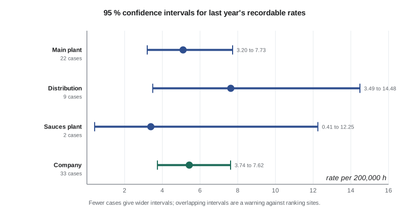
The intervals changed several conversations. The Dartmouth site's rate of 7.63 looked much worse than the main plant's 5.10, but its interval, 3.49 to 14.48, overlapped the main plant's almost entirely. One year's data could not show that the Dartmouth site was more dangerous, though the higher rate among agency workers, the weak reporting and the forklift findings all pointed that way. The sauces plant's rate of 3.39 rested on two cases and was consistent with an underlying rate anywhere from 0.41 to 12.25. Calling it the safest site on that evidence was not justified.

Overlapping intervals do not prove that two rates are the same, and a formal comparison of two rates is a little more sensitive than eyeballing overlap. But the rule of thumb served the leadership team well: if two intervals overlap substantially, do not rank the sites on that number alone.

Control charts

Confidence intervals answer a question about one period. Managers usually want to know something different: has something changed? Control charts, developed by Walter Shewhart in the 1920s for manufacturing quality, answer that question by plotting a measure over time against limits that show the range of ordinary variation. Points inside the limits with no pattern are treated as noise, which Shewhart's followers called common-cause variation. Points outside the limits, or certain patterns inside them, are signals of special-cause variation, worth investigating.

For injury rates, where the hours worked change from month to month, the right chart is the u-chart. It plots the rate in each period, \(u_i = c_i / n_i\), where \(c_i\) is the number of cases and \(n_i\) is the exposure in units of 200,000 hours. The centre line is the average rate over a baseline period, and the limits for each period depend on its own exposure:

Rules for signals

A single point outside the limits is the most obvious signal, but charts with wide limits rarely produce one. Practitioners therefore use additional rules that detect smaller sustained shifts. The most widely used, from the Western Electric rules and their successors, include:

• One point above the upper limit or below the lower limit.
• A run of eight or more consecutive points on the same side of the centre line.
• A steady trend of six or more points rising or falling in a row.
• Two out of three consecutive points in the outer third of the band between the centre line and a limit.

Each extra rule adds sensitivity and also adds false alarms. Nina started with the first two rules and agreed with Elena that any signal would trigger a review, not a conclusion. A review would ask what had changed and whether the change in the numbers matched anything known on the floor.

How sensitive is a monthly chart?

To show the leadership team what a u-chart could and could not detect, Nina built a test. She simulated 24 months in which the true rate was steady for 18 months and then nearly doubled for the last six, set the limits from the first 18 months, and checked when the chart would signal.

# A u-chart of monthly recordable rates with limits that vary with hours
import math, random
random.seed(1010)

def poisson(lam):
    L, k, p = math.exp(-lam), 0, 1.0
    while True:
        p *= random.random()
        if p < L:
            return k
        k += 1

hours = [random.randint(92_000, 110_000) for _ in range(24)]
true_rate = [5.4] * 18 + [10.5] * 6          # risk rises in the last six months
cases = [poisson(r * h / 200_000) for r, h in zip(true_rate, hours)]

base = 18                                   # set limits from the first 18 months
u_bar = sum(cases[:base]) / (sum(hours[:base]) / 200_000)
print(f"center line: {u_bar:.2f} per 200,000 hours")
above = 0
for m, (c, h) in enumerate(zip(cases, hours), start=1):
    n = h / 200_000                          # exposure in units of 200,000 hours
    u = c / n
    ucl = u_bar + 3 * math.sqrt(u_bar / n)
    lcl = max(0.0, u_bar - 3 * math.sqrt(u_bar / n))
    above = above + 1 if u > u_bar else 0
    flag = "  above upper limit" if u > ucl else ""
    if above >= 8:
        flag += "  run of 8 above center"
    print(f"month {m:2d}: {c:2d} cases  u = {u:5.2f}  limits {lcl:4.2f} to {ucl:5.2f}{flag}")

center line: 4.66 per 200,000 hours
month  1:  3 cases  u =  5.99  limits 0.00 to 13.81
month  2:  6 cases  u = 10.96  limits 0.00 to 13.40
month  3:  2 cases  u =  4.22  limits 0.00 to 14.06
month  4:  2 cases  u =  3.79  limits 0.00 to 13.57
month  5:  3 cases  u =  5.65  limits 0.00 to 13.54
month  6:  2 cases  u =  3.79  limits 0.00 to 13.57
month  7:  3 cases  u =  6.16  limits 0.00 to 13.93
month  8:  1 cases  u =  2.07  limits 0.00 to 13.97
month  9:  2 cases  u =  3.76  limits 0.00 to 13.53
month 10:  1 cases  u =  2.03  limits 0.00 to 13.87
month 11:  3 cases  u =  6.28  limits 0.00 to 14.02
month 12:  1 cases  u =  1.84  limits 0.00 to 13.44
month 13:  0 cases  u =  0.00  limits 0.00 to 13.44
month 14:  3 cases  u =  5.79  limits 0.00 to 13.65
month 15:  2 cases  u =  3.97  limits 0.00 to 13.77
month 16:  4 cases  u =  8.27  limits 0.00 to 13.96
month 17:  2 cases  u =  3.82  limits 0.00 to 13.60
month 18:  3 cases  u =  5.57  limits 0.00 to 13.48
month 19:  3 cases  u =  5.77  limits 0.00 to 13.63
month 20:  7 cases  u = 12.84  limits 0.00 to 13.42
month 21:  1 cases  u =  2.12  limits 0.00 to 14.07
month 22:  5 cases  u = 10.81  limits 0.00 to 14.18
month 23:  6 cases  u = 10.98  limits 0.00 to 13.41
month 24:  9 cases  u = 16.52  limits 0.00 to 13.42  above upper limit

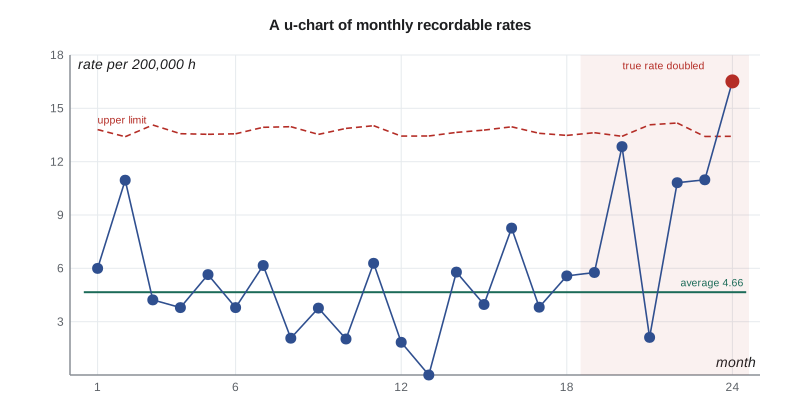
The result made the point better than any lecture. The true rate nearly doubled from month 19, but only month 24 fell above the upper limit. The run rule did not fire either, because month 21 happened to have a single case and fell below the centre line. A monthly injury chart for a company of Harrowgate Foods Ltd.'s size is a slow and blunt instrument. It will catch a large sustained change eventually, and it will stop managers from reacting to ordinary months. It will not give early warning.

That conclusion did not make the chart useless. It changed what it was used for. The u-chart became the standard way to show injury rates to the executive team and the board, with the explicit message that points inside the limits were not news. Early warning would have to come from the leading indicators, which change faster because they measure more frequent events, such as verifications and near misses. Nina built control charts for those too: a p-chart, the version for proportions, for critical control verification pass rates, and a u-chart for SIF-potential events.

Common mistakes with statistics

Statistical tools can be misused as easily as raw numbers. Elena added three warnings to the reporting guide. First, limits should be set from a stable baseline period and not recalculated every month, or a slow deterioration will drag the limits along with it. Second, a chart that never signals is not proof that nothing has changed; it may simply be too insensitive, as the simulation showed. Third, statistics cannot fix bad data. A falling rate caused by under-reporting will look like a genuine improvement on a control chart, which is why the reporting health ratios from Lesson 3 were plotted alongside the rates.