
GEOM-320 · Lesson 12 of 12 · 24 min
Applications: environment, agriculture and disasters
At the end of the second season Ruth asked Leah to write the program report for the district's board: what the monitoring had delivered, how well it had worked, what it had cost and what should change. The season had tested every part of the program. A June rain-on-snow event flooded the river bottomland below the headworks, a grass fire burned along the canal in August, the crop map and water use estimates were used to revise water allocations, and the InSAR results on the coulee banks led to a decision about the two moving sections. This lesson surveys the main applications of remote sensing to agriculture, the environment and disasters through that season, and closes the course with the design of an operational monitoring program.
Agriculture
Agriculture is one of the largest users of Earth observation. Crop type mapping, as in Lesson 7, supports statistics, insurance, water allocation and policy. Crop condition monitoring tracks vegetation indices against the average for the date and flags fields or regions below normal. Yield estimation relates the seasonal course of indices, especially their peak and integral, to yield through empirical models calibrated with harvest records, or assimilates satellite data into crop growth models. Precision agriculture uses within-field variation in images to define management zones for variable-rate seeding, fertilizer and irrigation. Irrigation mapping identifies irrigated land from greenness and moisture during dry periods and from the circular patterns of pivots; irrigation water use is estimated from ET, as in Lesson 10, or from crop coefficients and reference ET.
The crop coefficient approach estimates crop ET as \(ET_c = K_c \cdot ET_o\), where \(ET_o\) is the reference ET for a well-watered grass surface computed from weather data with the FAO Penman-Monteith equation, and \(K_c\) depends on the crop and its growth stage. Satellite data enter in two ways: the crop map gives the area of each crop, and the vegetation index of each field adjusts \(K_c\) to its actual canopy, since \(K_c\) rises roughly linearly with fractional cover. Net irrigation demand is ET minus effective rainfall, and the water the canal must deliver also covers losses in conveyance and application.
import math, random
random.seed(12)
# 1. Flood mapping from C-band backscatter (dB): open water is dark, fields are brighter
px = [random.gauss(-21.0, 1.8) for _ in range(1800)] + [random.gauss(-11.5, 2.2) for _ in range(6200)]
lo, hi = -30.0, 0.0; nb = 60
hist = [0] * nb
for v in px:
    i = int((min(max(v, lo), hi - 1e-9) - lo) / (hi - lo) * nb); hist[i] += 1
mid = [lo + (i + 0.5) * (hi - lo) / nb for i in range(nb)]
best = (0.0, None); tot = len(px); sum_all = sum(h * m for h, m in zip(hist, mid))
w0 = 0; s0 = 0.0
for i in range(nb - 1):
    w0 += hist[i]; s0 += hist[i] * mid[i]
    w1 = tot - w0
    if w0 == 0 or w1 == 0: continue
    m0 = s0 / w0; m1 = (sum_all - s0) / w1
    between = w0 * w1 * (m0 - m1) ** 2
    if between > best[0]: best = (between, (mid[i] + mid[i + 1]) / 2)
thr = best[1]
water = sum(1 for v in px if v < thr)
print(f"Otsu threshold {thr:.1f} dB; water pixels {water} of {tot}")
print(f"flooded area {water * 30 * 30 / 1e4:.1f} ha with 30 m pixels (true simulated water 1800 px = {1800 * 0.09:.1f} ha)")

# 2. Irrigation demand from mapped crop areas: ETc = Kc * ETo, net of effective rainfall, for July
ETo, rain_eff = 6.1, 0.9                 # mm/day reference ET, mm/day effective rainfall
crops = {"alfalfa": (6057, 1.15), "wheat": (9842, 1.10), "canola": (3200, 1.05), "potatoes": (1400, 1.10)}
tot_m3 = 0.0
print("\ncrop       area ha   Kc   net demand mm/d   July volume (1000 m3)")
for k, (a, kc) in crops.items():
    net = max(0.0, kc * ETo - rain_eff)
    vol = net / 1000 * a * 1e4 * 31
    tot_m3 += vol
    print(f"{k:9s} {a:8.0f}  {kc:4.2f}     {net:6.2f}           {vol / 1000:9.0f}")
print(f"total net July demand {tot_m3 / 1e6:.1f} million m3; at 75 % application efficiency the canal must deliver {tot_m3 / 0.75 / 1e6:.1f} million m3")
print(f"average canal flow needed {tot_m3 / 0.75 / (31 * 86400):.1f} m3/s")

# 3. Burned area by dNBR class (pixel counts from a grass fire next to the canal)
counts = {"unburned (< 0.10)": 2410, "low (0.10-0.27)": 1630, "moderate-low (0.27-0.44)": 720,
          "moderate-high (0.44-0.66)": 210, "high (> 0.66)": 35}
print()
for k, v in counts.items(): print(f"{k:28s} {v * 0.09:7.1f} ha")
print(f"burned area (low and above) {sum(v for k, v in counts.items() if not k.startswith('un')) * 0.09:.1f} ha")Otsu threshold -16.0 dB; water pixels 1922 of 8000 flooded area 173.0 ha with 30 m pixels (true simulated water 1800 px = 162.0 ha) crop area ha Kc net demand mm/d July volume (1000 m3) alfalfa 6057 1.15 6.11 11482 wheat 9842 1.10 5.81 17726 canola 3200 1.05 5.50 5461 potatoes 1400 1.10 5.81 2522 total net July demand 37.2 million m3; at 75 % application efficiency the canal must deliver 49.6 million m3 average canal flow needed 18.5 m3/s unburned (< 0.10) 216.9 ha low (0.10-0.27) 146.7 ha moderate-low (0.27-0.44) 64.8 ha moderate-high (0.44-0.66) 18.9 ha high (> 0.66) 3.1 ha burned area (low and above) 233.5 ha
The July demand computed in the code, from the estimated crop areas of Lesson 7 and a reference ET of 6.1 mm per day, is about 37 million cubic metres net and about 50 million cubic metres at 75 % application efficiency, an average canal flow of about 18.5 m³/s for the month. Compared with the district's diversion records, the estimate helped identify which laterals were delivering more than their fields needed and which fell short in the hottest weeks.
Worked problem
Field water demand
A 64 ha alfalfa field with full cover has \(K_c\) = 1.15. Reference ET is 6.1 mm per day and effective rainfall 0.9 mm per day. What net volume does the field need in a 10-day period, and what gross volume at 80 % application efficiency?
Show solution
- \[ET_c = 1.15 \times 6.1 = 7.02 \text{ mm/day}, \quad \text{net} = 7.02 - 0.9 = 6.12 \text{ mm/day}\]
- \[V_{net} = 0.00612 \text{ m} \times 640{,}000 \text{ m}^2 \times 10 = 39{,}170 \text{ m}^3\]
- \[V_{gross} = \frac{39{,}170}{0.80} = 48{,}960 \text{ m}^3\]
Answer: The field needs about 39,000 m³ net and about 49,000 m³ delivered at the pivot over ten days, roughly 57 L/s of continuous flow.
Environment
Environmental applications are as varied as the environment. Land cover mapping and monitoring underpins assessments of habitat, carbon and land use change. Wetland mapping combines optical data with radar, which detects water beneath vegetation through double bounce. Water quality monitoring estimates chlorophyll, turbidity and suspended sediment in lakes and reservoirs from visible and NIR reflectance, and detects harmful algal blooms; the district's reservoirs could be screened weekly for blooms that affect stock watering. Snow cover and snow water equivalent, mapped with optical and microwave sensors, feed forecasts of spring runoff that set the irrigation supply. Drought monitoring combines vegetation indices, land surface temperature, soil moisture from microwave sensors and precipitation.
In Canada, the Canadian Drought Monitor, coordinated by Agriculture and Agri-Food Canada, combines such indicators with reports from the ground to classify drought each month; the district's own maps of crop stress gave a local view consistent with that classification. Grassland and riparian areas along the coulees, important for wildlife, were mapped with the same Sentinel-2 time series as the crops and monitored for encroachment and invasive species.
Disasters
Remote sensing supports every phase of disaster management: mitigation and preparedness, through hazard mapping such as floodplain and wildfire fuel maps; response, through rapid maps of the extent of floods, fires and damage; and recovery, through monitoring of rebuilding and revegetation. During response, speed and reliability matter more than refinement. Radar is the primary tool for floods because floods come with cloud; open water appears dark, and a threshold on backscatter, chosen automatically from the histogram by a method such as Otsu's, separates water from land. Flooded vegetation and urban flooding are harder, because they can appear bright rather than dark, and need change detection against a pre-flood image or interferometric coherence.
Worked problem
Otsu threshold for flood mapping
The code applies Otsu's method to a histogram of 8,000 C-band pixels in dB. What does the method choose, and how does the mapped area compare with the true area?
Show solution
- \[\text{threshold maximizing between-class variance} = -16.0 \text{ dB}\]
- \[\text{water pixels} = 1922, \quad \text{area} = 1922 \times 0.09 = 173.0 \text{ ha}\]
- \[\text{true area} = 1800 \times 0.09 = 162.0 \text{ ha}, \quad \text{error} = +6.8 \%\]
Answer: The automatic threshold overestimates the water area by about 7 % because the tails of the land and water distributions overlap. Field reports and optical images, when available, are used to check and refine the extent.
In June, the rain-on-snow event raised the Oldman River and flooded the bottomland below the headworks. Natural Resources Canada's Emergency Geomatics Service produced flood extent products from RCM imagery for the provincial emergency agency, and Leah overlaid them on the district's infrastructure to check the intake, the access road and two pump stations. The district's own Sentinel-1 analysis added an image two days later showing the water receding. For major disasters, the International Charter on Space and Major Disasters, of which the Canadian Space Agency is a member, provides free satellite data from many agencies to authorized users.
The August grass fire was mapped as in Lesson 8. The burned area by dNBR class, in the code, totalled about 230 ha, mostly of low severity on grass, with small areas of high severity in the shelterbelt. Active fire detections from polar orbiting and geostationary weather satellites are available within minutes to hours of the satellite pass and are used by fire agencies to track large fires; for a fire of a few hundred hectares they gave an early alert but no useful detail. The canal right-of-way slowed the fire, and the severity map guided the reseeding of the bank.
The coulee banks
The InSAR monitoring of the coulee banks over two seasons showed that one of the two cracked sections was moving at about 15 to 20 mm per year along the line of sight, steadily, with no acceleration, while the other had stopped after the first spring. The inclinometers confirmed a shallow slip surface at the moving section. On the strength of these results the consultant recommended a drainage blanket and regrading at the moving section rather than relining a longer reach, and the board approved the work. The InSAR monitoring would continue to check whether the remedy worked. Ruth noted in the report that the decision rested on three independent kinds of evidence, satellite, inclinometer and survey, not on any one of them.
Designing an operational program
An operational program differs from a research project in its need for reliability, repeatability and accountability. Its design starts from the decisions it supports, not from the data available: what the users will do differently because of each product, how quickly they need it and how accurate it must be. From those requirements follow the data sources, the processing chain, the validation, the format of products and the schedule. The program must also plan for failure: a satellite can be lost, a data portal can change its formats, cloud can persist for weeks and key staff can leave, so every product needs a backup source and documented procedures.
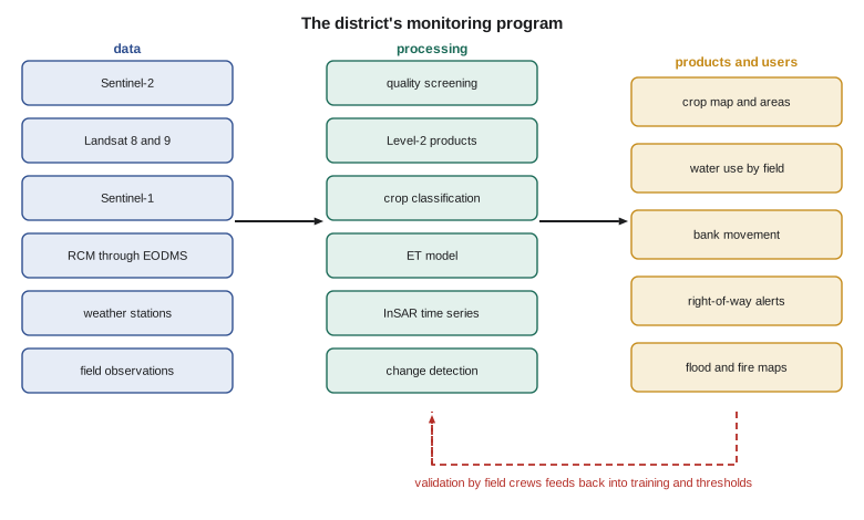
| Product | Decision supported | Frequency | Accuracy reported | Backup source |
|---|---|---|---|---|
| Crop map and areas | Water allocation, planning | Annual, provisional in July | Error matrix and area intervals | Landsat if Sentinel-2 is unavailable |
| Irrigation status and crop stress | Operations, lateral scheduling | Every clear pass, summary weekly | Field checks of flagged fields | Sentinel-1 backscatter |
| Water use (ET) by field | Allocation review, efficiency | Weekly in summer | Comparison with stations and deliveries | Crop coefficient method |
| Bank movement | Geotechnical decisions | Monthly | Comparison with inclinometers and reflector surveys | Second radar mission |
| Right-of-way change alerts | Maintenance and enforcement | Every 2 weeks | Inspection outcomes | Commercial imagery |
| Flood and fire maps | Emergency response | Within a day during events | Field reports | Emergency agency products |
Cost was the board's other question. Almost all imagery was free; the costs were staff time, computing, field work and the occasional purchase. The season's field work, about 300 field visits and the reflector surveys, cost as much as all the processing, and Leah argued that it was the best value in the program, because without it no product would have had a defensible accuracy. She recommended continuing it, together with a modest budget for commercial imagery in emergencies and a second airborne thermal survey after the embankment repairs.
Ethics, privacy and communication
Satellite images of farms are images of people's livelihoods. The district's maps showed the crops, irrigation and water use of individual farmers, information with commercial and personal value. The program's data policy, agreed with the board, limited field-level products to district staff and to each farmer for their own fields, published only aggregated results, and stated how long data would be kept. Products used to enforce rules, such as right-of-way encroachment, would always be confirmed by an inspection before any action. These principles follow the same professional obligations that apply to surveys: to report accurately, to state uncertainty, to protect the information entrusted to the engineer and to serve the public interest.
Communicating uncertainty to non-specialists is part of the work. A map with an accuracy of 89 % is wrong about one field in nine, and a board member who finds the error on their own field will doubt everything else unless the uncertainty was explained beforehand. Leah's report gave every product with its accuracy in plain words, maps of confidence where possible and a short explanation of what each product could and could not support.
Common mistakes
MistakeStarting a program from the data available rather than the decisions to be made.
InsteadDefine each product by the decision it supports, its timing and its needed accuracy.
MistakeRelying on a single satellite source.
InsteadPlan a backup source and procedure for every product.
MistakeCutting field work to save money.
InsteadField validation is what makes every product defensible; budget for it.
MistakeUsing remote sensing results alone for enforcement.
InsteadConfirm by inspection before acting on an alert.
MistakePublishing field-level data about individual farms without agreement.
InsteadAgree a data policy that protects individual information and aggregates public results.
Summary and key terms
- Agricultural applications include crop mapping, condition, yield, precision agriculture, irrigation mapping and water use.
- Crop ET can be estimated with crop coefficients adjusted by vegetation indices or by energy balance models.
- Environmental applications include land cover, wetlands, water quality, snow and drought.
- Radar is the primary tool for flood mapping; automatic thresholds such as Otsu's separate water from land.
- Fire mapping uses active fire detections for alerts and dNBR for severity after the fire.
- InSAR, combined with ground instruments, supports geotechnical decisions.
- Operational programs are designed from decisions, with backup sources, validation, documentation and a data policy.
- Crop coefficient
- The ratio of a crop's ET to reference ET at a given growth stage.
- Reference evapotranspiration
- The ET of a hypothetical well-watered grass surface computed from weather data.
- Otsu's method
- An automatic threshold that maximizes the between-class variance of a histogram.
- Active fire detection
- The identification of burning fires from thermal and midwave infrared satellite observations.
- International Charter on Space and Major Disasters
- An agreement among space agencies to provide satellite data free during major disasters.
- Operational program
- A monitoring system that delivers defined products reliably and repeatedly to users.
Practice problems
Work each problem on paper first, then reveal the answer to check.
A wheat field has K_c = 1.10 and ET_o = 5.5 mm/day. What is ET_c?
Show answer
6.05 mm/day.
Mapped flood water covers 2,400 pixels of 30 m. What is the area?
Show answer
2,400 × 0.09 ha = 216 ha.
A district needs 40 million m³ net in a 31-day month at 75 % efficiency. What average flow is needed?
Show answer
40 × 10⁶ / 0.75 / (31 × 86,400) = 19.9 m³/s.
Why is radar preferred to optical imagery during floods?
Show answer
Floods come with cloud, which radar penetrates, and radar works at night.
Give one reason a remote sensing alert should be confirmed before enforcement.
Show answer
Every product has errors; a false alarm could lead to an unjust action.
Lesson quiz · 5 questions
Score 60% or more to complete this lesson.
Create a free account to save your progress, take quizzes and earn a certificate.