Machine learning for remote sensing

By the second season Theo had moved the crop classification from maximum likelihood on a few dates to a random forest on a full season of Sentinel-2 indices, and reported an accuracy of 97 % from cross-validation. Leah was suspicious: the field validation the year before had given 89 %, and nothing in the method explained such a jump. Re-running the test with whole fields held out gave 87 %. The random forest was a better classifier, but not by as much as the first test claimed. This lesson introduces the machine learning methods now standard in remote sensing, from k-nearest neighbours and random forests to deep convolutional networks and foundation models, and the principles of training, validation and interpretation that decide whether their results can be trusted.

Why machine learning

Classical statistical classifiers such as maximum likelihood assume that each class follows a known distribution, usually normal. Real classes in multi-date, multi-sensor feature spaces are often multimodal, skewed and correlated in complex ways: wheat sown early and wheat sown late are two clusters, not one; a canola field before and after flowering occupies different regions. Machine learning classifiers learn decision boundaries directly from training data without assuming a distribution, can use dozens or hundreds of features of different kinds, such as reflectances, indices, radar backscatter, texture and terrain, and generally give higher accuracy when enough good training data are available. Their main risk is the same as that of every supervised method, only larger: they learn whatever is in the training data, including its biases and its spatial structure.

Classical machine learning methods

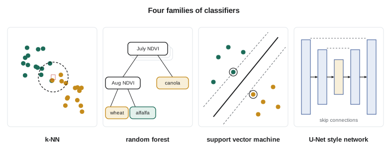
The k-nearest neighbours (k-NN) classifier assigns a pixel to the majority class among the k training samples nearest to it in feature space. It is simple and makes no assumptions about class shapes, but it is slow for large training sets, sensitive to the scaling of features and to irrelevant features, and it simply memorizes the training data.

Decision trees split the feature space with a sequence of thresholds on single features, chosen at each step to make the resulting groups as pure as possible by a measure such as the Gini index or entropy. A single tree is easy to interpret but unstable and prone to overfitting. A random forest grows many trees, each on a bootstrap sample of the training data and considering a random subset of features at each split, and classifies by majority vote. The randomization decorrelates the trees, so their combined vote is far more stable and accurate than any single tree. Random forests handle many features, are robust to noise and to features with different scales, need little tuning, and provide out-of-bag error estimates and measures of feature importance. They have become the default classifier for land cover and crop mapping. Gradient boosting builds trees in sequence, each correcting the errors of the previous ones, and often gives slightly higher accuracy with more tuning.

Support vector machines find the boundary between classes that maximizes the margin to the nearest training samples, the support vectors, and with kernel functions they can draw curved boundaries in the original feature space. They work well with small training sets in high-dimensional spaces, such as hyperspectral data, but are slower to train on large datasets and require choosing the kernel and its parameters.

Deep learning

Deep neural networks learn their own features from raw data. Convolutional neural networks (CNNs) apply many layers of learned filters to image patches, building up from edges and textures in the first layers to complex patterns such as field shapes, pivots and buildings in deeper layers. For semantic segmentation, the assignment of a class to every pixel, encoder-decoder architectures such as U-Net combine a contracting path that captures context with an expanding path that restores spatial detail. Recurrent networks and temporal attention models, including transformers, learn from time series of observations and are well suited to crop classification, where the sequence of growth stages is the strongest signal. Object detection networks find and outline individual objects such as centre pivots, grain bins and canal structures.

Deep learning has transformed tasks that depend on spatial patterns, such as mapping field boundaries, buildings and roads from high-resolution imagery, where classical pixel-based methods struggle. Its demands are large: thousands to millions of labelled examples, substantial computing resources, and careful design to avoid overfitting. Pretrained models reduce the demand: a network trained on a large dataset can be fine-tuned with a much smaller local one. Since 2023 several geospatial foundation models have been released, trained by self-supervised learning on very large archives of satellite imagery such as Landsat and Sentinel-2 and intended to be fine-tuned for tasks such as crop mapping, flood mapping and burn scar detection with modest amounts of labelled data. Their performance varies by task and region, and they still need local validation.

Training data at scale

Machine learning shifts the bottleneck from algorithms to labels. Sources of labels include field surveys, farmer and insurance records, visual interpretation of high-resolution imagery, existing maps such as national crop inventories, and crowd-sourced data. Each has its own errors. Labels transferred from an existing map inherit its mistakes and its legend; labels from the previous year are wrong wherever the crop rotated; labels digitized from imagery reflect the interpreter's skill and the image date. Class imbalance is common: in the service area, wheat and fallow fields far outnumber potatoes and sugar beets, and a classifier trained on the natural proportions tends to under-predict rare classes. Balanced sampling, class weights and careful reporting of per-class accuracy help.

Data augmentation, such as rotating and flipping image patches or adding noise, enlarges training sets for deep learning, but augmentations must respect the physics: flipping a patch is harmless, while altering spectral values arbitrarily can teach the model false relationships. Active learning selects the most informative unlabelled samples for an analyst to label next, reducing the effort needed. Labels must be documented with their source, date and confidence so that their quality can be judged later.

Validation and spatial autocorrelation

The central lesson of Theo's 97 % is that validation must reflect how the model will be used. Pixels close together are similar, a property called spatial autocorrelation: pixels from the same field share the same crop, soil, sowing date and management. If training and test pixels are drawn at random from the same fields, the test pixels have near-identical neighbours in the training set, and the model can score well by recognizing the field rather than the crop. When the model is applied to new fields, as it will be, accuracy is lower. The remedy is to split by spatial blocks: hold out whole fields, or whole areas, so that test samples are as independent of training samples as new fields will be. When the map is to be applied in a different year, testing on a held-out year gives the honest estimate.

import random, math
random.seed(11)
# Simulated training data: 24 fields, 15 pixels each; features are NDVI in June, July, August.
# Pixels within a field are very similar (spatial autocorrelation).
crops = {"alfalfa": (0.70, 0.80, 0.62), "wheat": (0.62, 0.78, 0.30), "canola": (0.45, 0.76, 0.40)}
fields = []
for fid in range(24):
    crop = list(crops)[fid % 3]
    base = [m + random.gauss(0, 0.07) for m in crops[crop]]          # field-to-field variation
    px = [[b + random.gauss(0, 0.015) for b in base] for _ in range(15)]  # pixel noise inside the field
    fields.append((fid, crop, px))

def dist(a, b): return math.sqrt(sum((x - y) ** 2 for x, y in zip(a, b)))
def knn(train, x, k=5):
    near = sorted(train, key=lambda t: dist(t[0], x))[:k]
    votes = {}
    for f, c in near: votes[c] = votes.get(c, 0) + 1
    return max(votes, key=votes.get)

# A tiny random forest of depth-2 trees on bootstrap samples with random features
def gini(rows):
    n = len(rows); counts = {}
    for _, c in rows: counts[c] = counts.get(c, 0) + 1
    return 1 - sum((v / n) ** 2 for v in counts.values())
def majority(rows):
    counts = {}
    for _, c in rows: counts[c] = counts.get(c, 0) + 1
    return max(counts, key=counts.get)
def best_split(rows, feats):
    best = None
    for f in feats:
        for t in sorted(set(round(r[0][f], 2) for r in rows)):
            L = [r for r in rows if r[0][f] <= t]; R = [r for r in rows if r[0][f] > t]
            if not L or not R: continue
            g = (len(L) * gini(L) + len(R) * gini(R)) / len(rows)
            if best is None or g < best[0]: best = (g, f, t, L, R)
    return best
def tree(rows, depth):
    if depth == 0 or gini(rows) == 0: return majority(rows)
    s = best_split(rows, random.sample(range(3), 2))
    if s is None: return majority(rows)
    return (s[1], s[2], tree(s[3], depth - 1), tree(s[4], depth - 1))
def predict(t, x):
    while isinstance(t, tuple): t = t[2] if x[t[0]] <= t[1] else t[3]
    return t
def forest(train, ntree=25):
    return [tree([random.choice(train) for _ in train], 2) for _ in range(ntree)]
def vote(F, x):
    v = {}
    for t in F: p = predict(t, x); v[p] = v.get(p, 0) + 1
    return max(v, key=v.get)

def evaluate(split):
    hits = {"k-NN": 0, "forest": 0}; total = 0
    for test_ids in split:
        train = [(p, c) for fid, c, px in fields if fid not in test_ids for p in px]
        test = [(p, c) for fid, c, px in fields if fid in test_ids for p in px]
        F = forest(train)
        for p, c in test:
            hits["k-NN"] += knn(train, p) == c; hits["forest"] += vote(F, p) == c
        total += len(test)
    return {k: v / total for k, v in hits.items()}

# Random pixel folds: pixels of the same field fall in both training and test sets
allpix = [(fid, i) for fid in range(24) for i in range(15)]
random.shuffle(allpix)
hits = {"k-NN": 0, "forest": 0}
for f in range(4):
    test = set(allpix[f::4])
    train = [(px[i], c) for fid, c, px in fields for i in range(15) if (fid, i) not in test]
    tst = [(px[i], c) for fid, c, px in fields for i in range(15) if (fid, i) in test]
    F = forest(train)
    for p, c in tst:
        hits["k-NN"] += knn(train, p) == c; hits["forest"] += vote(F, p) == c
print("random pixel 4-fold CV:  " + ", ".join(f"{k} {v / 360:.3f}" for k, v in hits.items()))
# Field-blocked folds: whole fields are held out together
blocks = [set(range(f, 24, 4)) for f in range(4)]
acc = evaluate(blocks)
print("field-blocked 4-fold CV: " + ", ".join(f"{k} {v:.3f}" for k, v in acc.items()))

random pixel 4-fold CV:  k-NN 0.975, forest 0.925
field-blocked 4-fold CV: k-NN 0.867, forest 0.864

The simulation reproduces Theo's experience. Each field has its own NDVI profile, varying from the crop's typical profile by field-to-field differences larger than the variation between pixels within a field. With random pixel folds, k-NN reaches 97.5 % because every test pixel has 14 nearly identical neighbours from its own field in the training set; the random forest, which generalizes more, reaches 92.5 %. With whole fields held out, both fall to about 86 to 87 %, which is the accuracy to expect on new fields. The gap between the two kinds of test is a measure of how much the random test overstated the accuracy. In this simulation the forest and k-NN perform similarly once tested honestly, a reminder that a sophisticated model is not automatically a better one.

Interpreting models

A classifier that cannot explain itself is hard to trust when it disagrees with an agronomist. Feature importance measures from random forests, such as the decrease in accuracy when a feature's values are randomly permuted, show which dates and bands drive the classification; in the district's model the most important features were the NDVI in mid-July, when canola flowers and wheat heads out, and the SWIR reflectance in early August, when the cereals ripen. Partial dependence plots show how the predicted probability of a class changes with one feature. For deep networks, saliency maps highlight the pixels that most influenced a prediction. These tools help detect when a model has learned something spurious, such as a road pattern that happened to coincide with one crop in the training data.

Models also need calibrated confidence. A classifier's output scores can be turned into probabilities and mapped alongside the class, so that users can see where the map is uncertain. Where the image contains conditions the model never saw in training, such as a new crop, unusual flooding or smoke, it will still produce a confident answer, and such areas must be flagged by checking how far each pixel is from the training data.

Operational practice

Leah's team adopted a set of rules for the machine learning work. Labels from field visits would be split by field, with a fixed held-out set never used for tuning. Accuracy would be reported from the held-out fields with the stratified estimators of Lesson 7. The previous year's model would be tested on the new year's fields before reuse, since conditions change between years. Training data, code, model versions and image lists would be kept so that every map could be reproduced. And any result that surprised an agronomist would be checked in the field before it was argued about in a meeting. Processing on cloud platforms that host the Landsat and Sentinel archives made it practical to train on full seasons of data for the whole service area in hours rather than weeks.