
GEOM-310 · Lesson 7 of 12 · 24 min
Aerial triangulation and bundle adjustment
The corridor strip contained 52 photos. Space resection of each one would have needed six control points per photo, more than three hundred painted targets along 24 km of farmland and coulee. Instead Grant's crew had surveyed twenty-four, and the aerial survey contractor delivered a single adjustment that oriented all 52 photos together, using thousands of tie points that the software had matched automatically between overlapping images. Theo was asked to review the adjustment report before the district accepted the orthophoto. This lesson explains what that report describes: block design and the points that tie it together, the history of aerial triangulation, the bundle adjustment and the structure of its equations, the roles of ground control and GNSS and IMU observations, self-calibration, blunder detection and the quality measures that tell a reviewer whether to trust the result.
Why triangulate
Aerial triangulation is the determination of the exterior orientation of a block of photos, and of the ground coordinates of points measured in them, from a limited amount of ground control. It extends control through the block in the way that a traverse or a GNSS network extends control between monuments. The photos are connected by tie points, natural features or matched image points that appear in two or more photos, and the whole block is fitted to the ground through control points and, in modern practice, through the measured positions and attitudes of the cameras. The result is a set of oriented photos ready for stereo compilation, surface generation and orthophoto production, and a set of ground coordinates for every tie point.
Block design
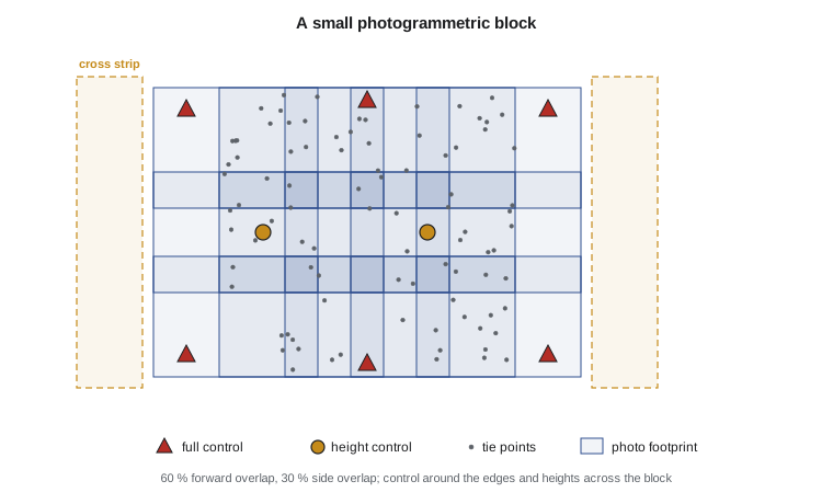
A block consists of one or more strips. Within a strip, consecutive photos overlap by 60 to 80 %; between strips, side overlap is 20 to 30 % for crewed aircraft and much larger for drones. Points in the central band of each photo appear in three consecutive photos in the same strip, and points in the side overlap appear in photos of two strips, up to six photos in total for traditional blocks. Classical practice placed tie points at six standard positions in each model, the von Gruber positions, near the top, centre and bottom of the overlap on both sides; automatic matching now produces hundreds or thousands of tie points per photo, which makes the block far stronger than any manual measurement could.
Control is placed according to the geometry of the block. Horizontal control is needed around the perimeter, because the block tends to drift and twist away from control like an unsupported traverse. Height control is needed across the block at intervals of a few models, because heights are the weakest part of the solution and a block of vertical photos tends to bend. Single strips, such as the canal corridor, are the weakest blocks of all: there is no side overlap to stiffen them, and errors in tilt about the flight line accumulate. The usual remedies are pairs of control points across the corridor at intervals along its length, cross strips flown perpendicular to the corridor at its ends and bends, and GNSS and IMU observations of the cameras.
From strips to bundles
Aerial triangulation began with analogue instruments that bridged control from one model to the next along a strip, accumulating errors that were corrected afterward by fitting polynomials to the control. Independent model triangulation formed and measured each stereo model separately and then joined all the models in a simultaneous three-dimensional similarity adjustment. Bundle adjustment, developed in the 1950s and 1960s and practical only with computers, treats the bundle of rays from each photo as the basic unit and adjusts all bundles together using the collinearity equations directly. It is the most rigorous method, because every image measurement enters the solution with its own weight and no intermediate products are formed, and it is now universal.
The bundle adjustment
In a bundle adjustment the unknowns are the six exterior orientation parameters of every photo and the three ground coordinates of every tie point, and optionally the interior orientation parameters and other systematic corrections. The observations are the image coordinates of every point in every photo in which it is measured, two collinearity equations each, together with the ground coordinates of control points, treated as weighted observations of their unknown coordinates, and, when available, the GNSS positions and IMU attitudes of the cameras. The linearized system is
The normal matrix has a strong structure. Each image point involves only one photo and one ground point, so \(\mathbf{N}_{22}\) is block-diagonal, with one 3 by 3 block per point, and \(\mathbf{N}_{11}\) has 6 by 6 blocks for each photo with coupling only between photos that share points. The point unknowns can be eliminated cheaply, leaving a reduced system for the photos alone,
which is much smaller than the full system. After solving for the photos, each point is found by back-substitution. This reduction, known as the Schur complement in linear algebra, is what makes bundle adjustments of thousands of photos and millions of points feasible, together with sparse matrix methods that exploit the fact that most photos share no points with each other.
Worked problem
Size of the corridor adjustment
The corridor block has 52 photos, 3000 tie points measured in an average of 3.2 photos each, 24 control points with all three coordinates, and GNSS positions and IMU attitudes for every photo. Count the observations, unknowns and redundancy, treating control coordinates as weighted unknowns.
Show solution
- \[\text{image observations} = 3000 \times 3.2 \times 2 = 19\,200\]
- \[\text{control observations} = 24 \times 3 = 72, \qquad \text{GNSS and IMU} = 52 \times 6 = 312\]
- \[\text{unknowns} = 52 \times 6 + (3000 + 24) \times 3 = 312 + 9072 = 9384\]
- \[r = 19\,200 + 72 + 312 - 9384 = 10\,200\]
Answer: The adjustment has more than ten thousand degrees of freedom. The reduced system for the photos alone is only 312 by 312, a trivial size for a computer, while the full normal matrix would be more than 9000 by 9000.
A small bundle adjustment
The program below adjusts three photos of a corridor strip with four control points at the corners and nine tie points, using the collinearity equations from Lesson 4, numerical partial derivatives and weighted least squares. Image coordinates have 3 µm noise and control coordinates 3 cm. It then repeats the adjustment with GNSS positions of the three exposure stations added as observations with 5 cm precision.
# A small bundle adjustment: three photos in a strip, four control points and nine tie points
import random
import math

def rot(om, ph, ka):
    """Photogrammetric rotation matrix M = R3(kappa) R2(phi) R1(omega), angles in degrees."""
    o, p, k = (math.radians(a) for a in (om, ph, ka))
    so, co, sp, cp, sk, ck = math.sin(o), math.cos(o), math.sin(p), math.cos(p), math.sin(k), math.cos(k)
    return [[cp * ck, co * sk + so * sp * ck, so * sk - co * sp * ck],
            [-cp * sk, co * ck - so * sp * sk, so * ck + co * sp * sk],
            [sp, -so * cp, co * cp]]

def project(eo, P, f):
    """Collinearity: ground point P = (X, Y, Z) -> image (x, y), same units as f."""
    XL, YL, ZL, om, ph, ka = eo
    M = rot(om, ph, ka)
    d = (P[0] - XL, P[1] - YL, P[2] - ZL)
    u, v, w = (sum(M[i][j] * d[j] for j in range(3)) for i in range(3))
    return -f * u / w, -f * v / w
def T(A): return [list(r) for r in zip(*A)]
def mul(A, B): return [[sum(a * b for a, b in zip(r, c)) for c in zip(*B)] for r in A]
def inv(A):
    n = len(A); M = [list(map(float, r)) + [1.0 if i == j else 0.0 for j in range(n)] for i, r in enumerate(A)]
    for c in range(n):
        p = max(range(c, n), key=lambda r: abs(M[r][c])); M[c], M[p] = M[p], M[c]
        d = M[c][c]; M[c] = [x / d for x in M[c]]
        for r in range(n):
            if r != c:
                f = M[r][c]; M[r] = [x - f * y for x, y in zip(M[r], M[c])]
    return [r[n:] for r in M]
def diag(v): return [[v[i] if i == j else 0.0 for j in range(len(v))] for i in range(len(v))]
def col(v): return [[x] for x in v]
random.seed(17)

ZREF = 900.0
f = 0.100; sig_img = 3.0e-6; sig_gcp = 0.03
true_eo = [[10000.0, 20000.0, ZREF + 2000.0, 0.40, -0.25, 0.30],
           [10520.0, 20012.0, ZREF + 2003.5, -0.35, 0.50, 0.10],
           [11040.0, 20021.0, ZREF + 1998.2, 0.20, 0.15, -0.20]]
grid = [(x, y) for x in (9930.0, 10520.0, 11110.0) for y in (19300.0, 20000.0, 20700.0)]
grid += [(10225.0, 19500.0), (10225.0, 20500.0), (10815.0, 19500.0), (10815.0, 20500.0)]
true_pts = [(x, y, ZREF + random.uniform(-30, 50)) for x, y in grid]
control = {0, 2, 6, 8}                               # the four corner points are ground control

obs = []                                             # (photo, point, x, y)
for i, eo in enumerate(true_eo):
    for j, P in enumerate(true_pts):
        x, y = project(eo, P, f)
        if abs(x) <= 0.0325 and abs(y) <= 0.050:
            obs.append((i, j, x + random.gauss(0, sig_img), y + random.gauss(0, sig_img)))
gcp_obs = {j: [c + random.gauss(0, sig_gcp) for c in true_pts[j]] for j in control}
sig_gnss = 0.05                                      # GNSS-measured exposure stations
gnss_obs = [[c + random.gauss(0, sig_gnss) for c in eo[:3]] for eo in true_eo]
print(f"{len(obs)} image points on 3 photos, {len(control)} control points, {len(true_pts) - len(control)} tie points")

# Unknowns: 6 per photo, then 3 per ground point
def unpack(p): return [p[6 * i:6 * i + 6] for i in range(3)], [p[18 + 3 * j:21 + 3 * j] for j in range(len(true_pts))]

def adjust(use_gnss, show):
    def model(p):
        eos, pts = unpack(p); out = []
        for i, j, _, _ in obs:
            out += list(project(eos[i], pts[j], f))
        for j in sorted(control):
            out += list(pts[j])
        if use_gnss:
            for eo in eos:
                out += list(eo[:3])
        return out
    lvec = [c for o in obs for c in o[2:]] + [c for j in sorted(control) for c in gcp_obs[j]]
    wts = [1.0] * (2 * len(obs)) + [(sig_img / sig_gcp) ** 2] * (3 * len(control))
    if use_gnss:
        lvec += [c for g in gnss_obs for c in g]; wts += [(sig_img / sig_gnss) ** 2] * 9
    # Approximations: the flight plan for the photos, a level-terrain projection for the points
    p = []
    for i in range(3):
        p += [10000.0 + 520.0 * i, 20000.0, ZREF + 2015.0, 0.0, 0.0, 0.0]
    for j, P in enumerate(true_pts):
        i, _, x, y = next(o for o in obs if o[1] == j)
        s = 2015.0 / f
        p += [10000.0 + 520.0 * i + s * x, 20000.0 + s * y, ZREF]
    n = len(p); step = [0.01, 0.01, 0.01, 1e-5, 1e-5, 1e-5] * 3 + [0.01] * (n - 18)
    for it in range(1, 9):
        m0 = model(p); w = [a - b for a, b in zip(lvec, m0)]
        J = [[0.0] * n for _ in w]
        for k in range(n):
            q = list(p); q[k] += step[k]; mk = model(q)
            for r in range(len(w)):
                J[r][k] = (mk[r] - m0[r]) / step[k]
        N = [[sum(wts[r] * J[r][a] * J[r][b] for r in range(len(w))) for b in range(n)] for a in range(n)]
        u = [[sum(wts[r] * J[r][a] * w[r] for r in range(len(w)))] for a in range(n)]
        Q = inv(N); dx = [d[0] for d in mul(Q, u)]
        p = [a + d for a, d in zip(p, dx)]
        big = max(abs(d) for k, d in enumerate(dx) if step[k] == 0.01)
        if show:
            print(f"iteration {it}: largest coordinate correction {big:9.4f} m")
        if big < 1e-4:
            break
    v = [a - b for a, b in zip(lvec, model(p))]
    dof = len(v) - n
    s0 = (sum(wt * r * r for wt, r in zip(wts, v)) / dof) ** 0.5
    eos, pts = unpack(p)
    ties = [j for j in range(len(true_pts)) if j not in control]
    if show:
        print(f"Redundancy {dof}; sigma0 = {1e6 * s0:.2f} microns (a priori 3.00)")
        print("Tie point     error X   error Y   error Z   sigma Z   seen on")
        for j in ties:
            e = [a - b for a, b in zip(pts[j], true_pts[j])]
            sz = s0 * Q[18 + 3 * j + 2][18 + 3 * j + 2] ** 0.5
            seen = sum(1 for o in obs if o[1] == j)
            print(f"  T{j + 1:<2d}       {e[0]:+7.3f}   {e[1]:+7.3f}   {e[2]:+7.3f}   {sz:7.3f}   {seen} photos")
    rz = (sum((pts[j][2] - true_pts[j][2]) ** 2 for j in ties) / len(ties)) ** 0.5
    rxy = (sum((pts[j][0] - true_pts[j][0]) ** 2 + (pts[j][1] - true_pts[j][1]) ** 2 for j in ties) / len(ties)) ** 0.5
    msz = sum(s0 * Q[20 + 3 * j][20 + 3 * j] ** 0.5 for j in ties) / len(ties)
    return rxy, rz, msz

print()
print("Control only:")
a = adjust(False, True)
b = adjust(True, False)
print()
print("Tie point accuracy      RMS horizontal   RMS vertical   mean sigma Z")
print(f"  4 GCPs only           {a[0]:10.3f} m   {a[1]:10.3f} m   {a[2]:9.3f} m")
print(f" 4 GCPs + GNSS stations {b[0]:10.3f} m {b[1]:10.3f} m {b[2]:9.3f} m")29 image points on 3 photos, 4 control points, 9 tie points Control only: iteration 1: largest coordinate correction 46.8348 m iteration 2: largest coordinate correction 4.0357 m iteration 3: largest coordinate correction 0.0081 m iteration 4: largest coordinate correction 0.0000 m Redundancy 13; sigma0 = 3.04 microns (a priori 3.00) Tie point error X error Y error Z sigma Z seen on T2 +0.077 -0.034 +0.186 0.372 2 photos T4 +0.002 +0.075 +0.522 0.350 3 photos T5 +0.001 +0.054 +0.313 0.245 3 photos T6 -0.091 +0.056 -0.121 0.344 3 photos T8 +0.077 +0.017 -0.071 0.394 2 photos T10 +0.036 +0.143 +0.341 0.410 2 photos T11 +0.044 -0.076 +0.249 0.398 2 photos T12 -0.030 -0.011 -0.030 0.410 2 photos T13 -0.031 +0.052 -0.005 0.407 2 photos Tie point accuracy RMS horizontal RMS vertical mean sigma Z 4 GCPs only 0.086 m 0.259 m 0.370 m 4 GCPs + GNSS stations 0.071 m 0.168 m 0.311 m
The adjustment converges in four iterations from approximate values tens of metres away. The estimated reference standard deviation of 3.04 µm matches the 3 µm noise that was simulated, which is the first check a reviewer makes. The tie points in the triple overlap, seen on three photos, have the smallest height uncertainty; those seen on only two photos near the ends of the strip are weaker. Even so, the height precision of about 0.37 m is poor for a 10 cm GSD project: the base-to-height ratio of 0.26 and the narrow single strip with control only at its ends limit what three photos can deliver. Adding the GNSS positions of the cameras reduces the vertical errors of the tie points from 0.26 to 0.17 m RMS and their expected height uncertainty from 0.37 to 0.31 m. In the full 52-photo corridor, with many more tie points per photo, multi-image rays and control pairs every few kilometres, the same principles give heights of a few centimetres to a decimetre.
Self-calibration and additional parameters
Bundle adjustments routinely estimate the camera calibration along with the orientations. The interior orientation parameters of Lesson 2 are added as unknowns, common to all photos taken with the same camera, and sometimes additional parameters are included to model systematic image errors not described by the standard distortion model. Self-calibration needs a geometry that separates the camera parameters from the orientation: control at a range of heights, cross strips, varying flying heights or convergent images. The adjustment report should show the estimated values, their standard deviations and their correlations; a focal length correlated at 0.99 with the average flying height has not been determined, whatever its standard deviation suggests.
GNSS and IMU in the adjustment
When camera positions and attitudes are observed, they enter the adjustment as additional observation equations linking the trajectory to the exterior orientation through the lever arm and boresight of Lesson 5. Typical additional unknowns are a constant offset of the GNSS positions for each strip, to absorb errors such as an incorrect antenna height or a datum shift, and the three boresight angles. With good GNSS and IMU data, control is needed mainly to define the datum and to check the result, and a block can be adjusted with a handful of control points instead of dozens. The control that is used should still be placed at the edges and corners, where the block would otherwise extrapolate.
Blunders and robust estimation
Automatic matching produces many tie points and a small percentage of wrong ones, from repetitive texture, moving vehicles, shadows that move between exposures or reflections from water. Manual measurement produces occasional blunders, such as a control target measured in the wrong place or labelled with the wrong number. Least squares spreads the effect of a blunder over many residuals, so blunders must be found and removed. Two approaches are used together. Statistical testing, known as data snooping, examines each standardized residual \(w_i = v_i / \sigma_{v_i}\) and rejects observations for which it exceeds a threshold, typically about 3 to 4, one at a time, re-adjusting after each rejection. Robust estimation reduces the weight of observations with large residuals automatically in each iteration, so that blunders lose their influence without being identified one by one.
Control points deserve special care because a single wrong control point can bend a whole block. A good practice is to adjust the block first with minimal control, so that the residuals at the remaining control points are true checks, and then to add the checked control. Points with large residuals should be investigated in the field records and the imagery rather than simply deleted: a target that was disturbed by a farmer's equipment between survey and flight is a fact about the project, not noise.
Reading an adjustment report
A reviewer looks at a short list of things. The reference standard deviation should match the expected image precision, a third to a half of a pixel for good imagery. Image residuals should be small, with no systematic pattern across the format; a radial pattern indicates a distortion problem. Control point residuals should be consistent with the control survey accuracy. The number of rays per tie point and the distribution of tie points should show that every photo is well connected. The standard deviations of the exterior orientations, the self-calibration parameters and their correlations should be reasonable. Most important, the checkpoints, surveyed points not used in the adjustment, should agree with the adjusted coordinates to within the specified accuracy. Lesson 12 describes how checkpoint statistics are computed and reported.
| Item in the report | Typical good value | What a bad value suggests |
|---|---|---|
| Reference standard deviation | One third to one half of a pixel | Blunders, wrong camera model or poor matching |
| Image residual pattern | Random over the format | Radial pattern: distortion; one corner: rolling shutter or film flatness |
| Control residuals | Within the control survey accuracy | Wrong target, disturbed target or datum error |
| Rays per tie point | Mostly 3 or more | Weak connections between photos or strips |
| Checkpoint RMSE | Within the specification | Systematic error not visible in the adjustment |
Theo's review found one problem. Control point 17, beside a field approach, had a vertical residual of 0.31 m while every other point was within 6 cm. The crew's photos showed that the target had been painted on a gravel pad that the farmer had regraded after the survey and before the flight. The point was removed from the control and reported as disturbed.
Common mistakes
MistakePlacing control only along the centre line of a corridor.
InsteadUse pairs of points across the corridor and cross strips to control tilt about the flight line.
MistakeAccepting the adjustment because the control residuals are small.
InsteadControl residuals can be small by construction; judge accuracy at independent checkpoints.
MistakeSelf-calibrating without checking correlations.
InsteadInspect correlations of camera parameters with orientation; strengthen the geometry if they approach 1.
MistakeDeleting control points with large residuals without investigation.
InsteadInvestigate field records and imagery; a disturbed or misidentified point is a fact to report.
MistakeIgnoring tie points seen in only two photos at the ends of strips.
InsteadAdd extra photos beyond the ends and cross strips so every area is seen by three or more photos.
Summary and key terms
- Aerial triangulation orients a block of photos from limited control using tie points and camera observations.
- Block design sets overlaps, strip layout and control distribution; single strips are the weakest blocks.
- Bundle adjustment uses the collinearity equations directly for all photos and points simultaneously.
- The normal matrix is sparse; eliminating the point unknowns leaves a small reduced system for the photos.
- GNSS and IMU observations reduce the need for control and stabilize heights; control still defines and checks the datum.
- Self-calibration estimates camera parameters but requires geometry that decorrelates them from the orientation.
- Blunders are found by data snooping or controlled by robust estimation; checkpoints are the final test.
- Aerial triangulation
- The determination of exterior orientation and tie point coordinates for a block of photos from limited control.
- Tie point
- A point measured in two or more photos that connects them in the adjustment.
- Bundle adjustment
- A simultaneous least-squares adjustment of all image rays using the collinearity equations.
- Reduced normal equations
- The smaller system for photo unknowns obtained by eliminating point unknowns.
- Data snooping
- Testing standardized residuals one at a time to detect blunders.
- Checkpoint
- A surveyed point not used in the adjustment, used to assess accuracy independently.
Practice problems
Work each problem on paper first, then reveal the answer to check.
A block has 120 photos and 8000 tie points, each in 4 photos on average, and 10 control points. How many image observations are there?
Show answer
8000 × 4 × 2 = 64 000.
Why is N22 block-diagonal in a bundle adjustment?
Show answer
Each image observation involves only one ground point, so different points are not coupled directly.
A standardized residual is 5.2 with a threshold of 3.3. What should be done?
Show answer
Flag the observation as a likely blunder, remove it and re-adjust, then check the next largest.
Why are extra photos taken beyond the ends of a strip?
Show answer
So that the end areas are seen in three photos and the end models are complete and well connected.
What does a radial pattern of image residuals suggest?
Show answer
An error or omission in the lens distortion model.
Lesson quiz · 5 questions
Score 60% or more to complete this lesson.
Create a free account to save your progress, take quizzes and earn a certificate.