
GEOM-310 · Lesson 3 of 12 · 24 min
Image coordinates
Theo Martel's order from the National Air Photo Library arrived as a set of high-resolution scans of 1962 photographs that covered the old canal alignment, together with a scan of the camera's calibration report. The district wanted the old alignment and the edge of the coulee as they were before sixty years of erosion, plotted in today's coordinates. Before any of that could happen, Theo had to answer a basic question: where, in millimetres relative to the principal point of the 1962 camera, is each pixel of the scan? The same question, in a simpler form, applies to every digital image from the corridor camera and the drone. This lesson covers image coordinate systems, the two-dimensional transformations that connect them, fiducial marks and scanned film, the measurement of image points, and the small systematic corrections for atmospheric refraction and Earth curvature.
Three coordinate systems
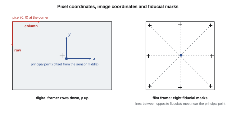
A digital image is an array of pixels addressed by column and row. The pixel coordinate system has its origin at the top-left corner of the image, the column number increasing to the right and the row number increasing downward. Conventions differ on whether the centre of the first pixel is at (0, 0) or at (0.5, 0.5); in this course the edge of the image is at 0 and the centre of the first pixel at 0.5, so a point measured at column 12.0 lies on the boundary between pixels 11 and 12. Off-by-half-pixel errors are among the most common bugs in photogrammetric software, and they are invisible until a careful check shows a systematic shift of half a GSD.
The image coordinate system used in the equations of photogrammetry is a right-handed system in the image plane, measured in millimetres, with its origin at the principal point, x increasing in the direction of flight (or to the right in the image) and y increasing upward. The z axis completes the right-handed system and points from the image toward the perspective centre, so the perspective centre has image-space coordinates \((x_p, y_p, f)\) and an image point \((x, y, 0)\). For a digital frame camera the connection between pixel and image coordinates is a fixed transformation: subtract half the image size, multiply by the pixel size, flip the sign of the row axis, and subtract the principal point offset.
where \(c\) and \(r\) are the column and row of the measured point counted from 0 at the image edge, \(N_c\) and \(N_r\) are the numbers of columns and rows, and \(p\) is the pixel size. The third system, the object or ground coordinate system, is where the answers are wanted; Lessons 4 and 5 connect image to ground.
Fiducial marks and scanned film
A film photograph has no pixels. Its coordinate system is defined by fiducial marks, small targets exposed onto every frame by the camera body, at the corners, at the midpoints of the sides, or both. The calibration report gives the calibrated coordinates of each fiducial relative to the principal point. When the film is processed, stored and scanned, the image is shifted, rotated, stretched slightly differently in the two directions by film shrinkage, and sampled by the scanner's own pixel grid. Interior orientation of a scanned photo is the process of measuring the fiducials in the scan and finding the transformation that carries scan coordinates to calibrated image coordinates.
The 1962 photographs were taken with a wide-angle survey camera of 152.4 mm nominal focal length and a 230 mm square format. The archive scanned them with 21 µm pixels, so each frame is about 11 000 pixels square and a pixel covers about 0.4 m on the ground at the 1:20 000 scale of the photography. The calibration report lists eight fiducials, four at the corners and four at the side midpoints, with calibrated coordinates to a micrometre.
Two-dimensional transformations
Three transformations are used between plane coordinate systems. The conformal, or similarity, transformation has four parameters: two translations, a rotation and one scale. It preserves shape and is appropriate when the two systems differ only by position, orientation and uniform scale. The affine transformation has six parameters: two translations, a rotation, two scales, and a non-orthogonality. It allows different scales in the two directions and a slight skew, which describes film shrinkage and many scanner errors well. The projective transformation has eight parameters and describes the relation between two planes viewed in central projection: a tilted photo of flat ground, for example, or a photo and a planar façade. It is used in rectification, not in interior orientation.
Each fiducial gives two equations in the six affine unknowns, so three fiducials determine the transformation exactly and the remaining five of the eight give redundancy. Least squares, from GEOM-220, gives the best estimate, and the residuals show the quality of the measurements and the suitability of the model: residuals of a few micrometres are normal for a good scan; residuals of tens of micrometres point to a misidentified fiducial, a damaged film or a scanner fault.
| Transformation | Parameters | Preserves | Typical use |
|---|---|---|---|
| Conformal (similarity) | 4: two shifts, rotation, scale | Shape and angles | Datum shifts, digitizer setup |
| Affine | 6: two shifts, rotation, two scales, skew | Parallel lines | Interior orientation of scanned film |
| Projective | 8 | Straight lines | Rectification of a plane, façades |
| Polynomial | 12 or more | Nothing in general | Empirical correction of local distortions |
The program below simulates Theo's measurement of the eight fiducials in the scan, including a small rotation of the photo on the scanner and slightly unequal scales, and fits the affine transformation. It then transforms a point measured on the coulee rim to image coordinates.
# Interior orientation of a scanned 1962 air photo: an affine fit to eight fiducials,
# then refraction and Earth curvature corrections for one image point
import math, random
random.seed(31)
ZREF = 900.0

# Calibrated fiducial coordinates from the camera calibration report (mm)
fid = [(-106.000, -106.000), (106.001, 105.998), (-105.999, 106.003), (106.002, -106.001),
       (-112.003, 0.002), (111.998, -0.001), (0.001, 112.002), (-0.002, -111.997)]

# The scanner (21 micron pixels) placed the photo slightly rotated, shifted and with
# unequal scales; generate the measured pixel positions of the fiducial marks
true = dict(a0=5701.3, a1=47.6012, a2=-0.1662, b0=5688.9, b1=-0.1667, b2=-47.5983)
meas = []
for x, y in fid:
    c = true['a0'] + true['a1'] * x + true['a2'] * y + random.gauss(0, 0.15)
    r = true['b0'] + true['b1'] * x + true['b2'] * y + random.gauss(0, 0.15)
    meas.append((c, r))

# Least squares for x = a0 + a1*c + a2*r and y = b0 + b1*c + b2*r (pixels -> mm)
def solve3(rows, obs):
    N = [[sum(ri[i] * ri[j] for ri in rows) for j in range(3)] for i in range(3)]
    u = [sum(ri[i] * o for ri, o in zip(rows, obs)) for i in range(3)]
    # Cramer's rule for the 3 x 3 normal equations
    det = lambda M: (M[0][0] * (M[1][1] * M[2][2] - M[1][2] * M[2][1])
                     - M[0][1] * (M[1][0] * M[2][2] - M[1][2] * M[2][0])
                     + M[0][2] * (M[1][0] * M[2][1] - M[1][1] * M[2][0]))
    D = det(N); out = []
    for k in range(3):
        Mk = [[u[i] if j == k else N[i][j] for j in range(3)] for i in range(3)]
        out.append(det(Mk) / D)
    return out

A = [(1.0, c, r) for c, r in meas]
ax = solve3(A, [x for x, _ in fid]); by = solve3(A, [y for _, y in fid])
print(f"x = {ax[0]:9.4f} {ax[1]:+.6f} c {ax[2]:+.6f} r")
print(f"y = {by[0]:9.4f} {by[1]:+.6f} c {by[2]:+.6f} r")
res = []
for (c, r), (x, y) in zip(meas, fid):
    res += [ax[0] + ax[1] * c + ax[2] * r - x, by[0] + by[1] * c + by[2] * r - y]
s0 = math.sqrt(sum(v * v for v in res) / (len(res) - 6))
print(f"Residual standard deviation {1000 * s0:.1f} microns from {len(res)} observations")
sx = math.hypot(ax[1], by[1]); sy = math.hypot(ax[2], by[2])
print(f"Scale x {1000 * sx:.3f} um/pixel   scale y {1000 * sy:.3f} um/pixel")

c, r = 9634.0, 3120.0       # a well-defined point on the coulee rim
x = ax[0] + ax[1] * c + ax[2] * r; y = by[0] + by[1] * c + by[2] * r
print(f"Point (c, r) = ({c:.0f}, {r:.0f}) -> x = {x:.3f} mm, y = {y:.3f} mm")

# Refraction (standard atmosphere model) and Earth curvature corrections
f = 152.400                 # mm, a wide-angle survey camera of the period
hk = (ZREF + 20.0) / 1000    # ground elevation at the point (km)
Hk = hk + 3.030              # flying altitude (km): 3030 m above the ground
K = (2410 * Hk / (Hk ** 2 - 6 * Hk + 250) - 2410 * hk ** 2 / ((hk ** 2 - 6 * hk + 250) * Hk)) * 1e-6
rad = math.hypot(x, y)
dr_ref = K * (rad + rad ** 3 / f ** 2)
dr_cur = rad ** 3 * (Hk - hk) * 1000 / (2 * 6371000 * f ** 2)     # f and rad in mm, H in m
print(f"Radial distance {rad:.3f} mm   K = {K * 1e6:.2f} x 10^-6")
print(f"Refraction moves the point outward by {1000 * dr_ref:.1f} um: correct inward")
print(f"Earth curvature moves it inward by {1000 * dr_cur:.1f} um: correct outward (map projection use)")x = -119.3541 +0.021008 c -0.000073 r y = 119.9375 -0.000074 c -0.021009 r Residual standard deviation 3.6 microns from 16 observations Scale x 21.008 um/pixel scale y 21.009 um/pixel Point (c, r) = (9634, 3120) -> x = 82.808 mm, y = 53.682 mm Radial distance 98.686 mm K = 37.25 x 10^-6 Refraction moves the point outward by 5.2 um: correct inward Earth curvature moves it inward by 9.8 um: correct outward (map projection use)
The residual standard deviation of about 3.6 µm, a sixth of a scanner pixel, shows that the fiducials were measured well and that the affine model fits. The two scale factors, 21.008 and 21.009 µm per pixel, differ by less than one part in twenty thousand here; differences of several parts in ten thousand are common for older film, which shrinks unevenly along and across the roll. The coefficients \(a_2\) and \(b_1\) of about \(-7 \times 10^{-5}\) correspond to a rotation of the photo on the scanner of about 0.2°.
Worked problem
An exact affine solution
Three fiducials have calibrated coordinates (−106, −106), (106, 106) and (−106, 106) mm and are measured in a scan at pixel positions (c, r) = (502, 10 594), (10 594, 502) and (502, 502). Assuming no rotation, find the affine scale factors and the shifts.
Show solution
- \[x: \; -106 = a_0 + 502\,a_1, \quad 106 = a_0 + 10\,594\,a_1 \;\Rightarrow\; a_1 = \frac{212}{10\,092} = 0.021007 \text{ mm/pixel}\]
- \[a_0 = -106 - 502 \times 0.021007 = -116.546 \text{ mm}\]
- \[y: \; 106 = b_0 + 502\,b_2, \quad -106 = b_0 + 10\,594\,b_2 \;\Rightarrow\; b_2 = -0.021007 \text{ mm/pixel}\]
- \[b_0 = 106 + 502 \times 0.021007 = 116.546 \text{ mm}\]
Answer: The scale is 21.007 µm per pixel in both directions, negative in y because rows increase downward while y increases upward. With only three points there is no redundancy and no check; the remaining fiducials provide it.
Measuring image points
Image points are measured in three ways. Manual measurement places a cursor on a feature in a single image or, better, in a stereo view; a trained operator can point to well-defined features to a fraction of a pixel. Targeted measurement uses specially placed targets, such as painted crosses or checkerboard panels on control points, whose centres can be found automatically by fitting a model to the pattern of brightness; precisions of a tenth of a pixel or better are typical for clean targets. Image matching finds the same feature in two or more images by comparing small windows of brightness values; it is the engine of automatic tie point measurement and dense surface generation.
Area-based matching compares a small template from one image with candidate positions in another and chooses the position that maximizes a similarity measure, commonly the normalized cross-correlation coefficient. Least-squares matching refines the position to a few hundredths of a pixel by solving for small shifts and distortions of the window. Feature-based matching, used in structure from motion, first detects distinctive points such as corners or blobs in each image independently, describes the neighbourhood of each point with a descriptor that is insensitive to rotation and scale, and then pairs descriptors between images. Lesson 8 describes feature-based matching in more detail.
The correlation coefficient \(\rho\) is 1 for identical windows and is insensitive to differences in brightness and contrast between images. It fails where there is no texture, as on calm water, fresh snow or a uniform concrete slab, and where the texture repeats, as in rows of crops or a field of identical roof panels. Matching software therefore checks matches for consistency, typically by matching in both directions and rejecting pairs that disagree.
Atmospheric refraction
Light from the ground travels through air whose density decreases with height, so the ray bends slightly, curving downward along its path. A ray reaching the camera at an angle from the vertical arrives from a direction slightly farther from the nadir than the straight line from the object, and the image point is displaced radially outward. For a standard atmosphere the displacement is
where \(H\) is the flying altitude and \(h\) the ground elevation, both in kilometres above sea level. The correction is applied inward. For high-altitude aerial photography it amounts to several micrometres at the edges of the format, comparable to the measurement precision of film; for drones flying 100 m above the ground it is negligible. Modern bundle adjustment software applies it automatically when the camera altitude is known, or absorbs it into self-calibration.
Earth curvature
If ground coordinates are expressed in a map projection with heights above the ellipsoid or geoid, the curved Earth is being treated as a plane. Points far from the nadir lie below that plane by about \(D^2 / 2R\), where \(D\) is the distance from the nadir and \(R\) the radius of the Earth, and they are imaged as if they had that negative height: displaced radially inward. The displacement is
and the correction is applied outward. It is not a property of the camera or the atmosphere but of the mixed coordinate system. When the photogrammetric computation is carried out in a three-dimensional Cartesian frame, such as a local tangent-plane system or earth-centred coordinates, there is no curvature correction to apply; the coordinates are transformed to the map projection afterward. Most modern software works this way for large projects, while some apply the correction for map projection coordinates. Mixing the two, by applying the correction in a Cartesian computation or omitting it in a map projection computation, produces height errors that grow with the square of the distance from the centre of the block.
For the 1962 photograph, flown about 3030 m above ground at the rim, the program finds a refraction displacement of about 5 µm outward and a curvature displacement of about 10 µm inward at a radial distance of 99 mm. Both are small compared with the 21 µm scanner pixel, but they are systematic, they act in the same radial direction on every photo, and over a block they would produce a measurable deformation of the coulee surface. Theo kept both corrections in his processing because the archival photography would be adjusted in projection coordinates tied to today's control.
Putting the corrections in order
For a scanned film photo, a measured point passes through a sequence of steps before it can be used in the collinearity equations: transform scan pixel coordinates to calibrated image coordinates with the affine transformation from the fiducials; reduce to the principal point; correct for lens distortion; correct for atmospheric refraction; and, if the object coordinates are in a map projection, correct for Earth curvature. For a digital frame camera the first step is the fixed pixel-to-image conversion, and the rest are the same. The order matters little for the small corrections but matters greatly for the first: distortion coefficients are defined in image coordinates relative to the principal point, not in pixel coordinates, and applying them in the wrong system gives wrong answers that look plausible.
Common mistakes
MistakeMixing pixel row direction with image y direction.
InsteadRows increase downward and y increases upward; one sign must change.
MistakeIgnoring the half-pixel offset between pixel edges and centres.
InsteadDecide the convention and apply it consistently; a mismatch shifts every point by half a GSD.
MistakeUsing a conformal transformation for scanned film.
InsteadFilm shrinks differently in the two directions; use an affine transformation.
MistakeApplying Earth curvature corrections in a Cartesian computation.
InsteadCurvature applies only when ground coordinates are a map projection treated as a plane.
MistakeTrusting a correlation match on uniform or repeating texture.
InsteadCheck matches in both directions and reject inconsistent ones.
Summary and key terms
- Pixel coordinates start at the image corner with rows downward; image coordinates start at the principal point with y upward.
- Film photographs are referred to calibrated fiducial marks; scanned photos need an affine transformation from scan to image coordinates.
- Conformal, affine and projective transformations have 4, 6 and 8 parameters and suit different relationships.
- Image points are measured manually, by fitting targets, or by image matching with correlation and least-squares refinement.
- Atmospheric refraction displaces points outward; the correction is applied inward.
- Earth curvature correction applies only to computations in map projection coordinates.
- Corrections are applied in image coordinates relative to the principal point, after the fiducial or pixel transformation.
- Pixel coordinates
- Column and row positions in a digital image, counted from the top-left corner.
- Image coordinates
- Plane coordinates in the image, in millimetres, relative to the principal point, with y upward.
- Fiducial marks
- Reference targets exposed on each film frame whose calibrated positions define the image coordinate system.
- Affine transformation
- A six-parameter plane transformation allowing different scales on two axes and a skew.
- Normalized cross-correlation
- A similarity measure between two image windows that ignores differences in brightness and contrast.
- Atmospheric refraction
- The bending of light rays in the atmosphere, which displaces image points radially outward.
Practice problems
Work each problem on paper first, then reveal the answer to check.
An image has 20 000 columns and 5 µm pixels with no principal point offset. What is x for column 15 000.0?
Show answer
x = (15 000 + 0.5 − 10 000) × 0.005 = 25.0025 mm.
How many fiducials are needed to determine an affine transformation, and how many give redundancy if eight are measured?
Show answer
Three determine it; with eight there are 16 − 6 = 10 redundant observations.
Why is correlation matching unreliable on a freshly graded gravel pad?
Show answer
The surface has little distinct texture, so many positions look alike.
At r = 100 mm, f = 152 mm, H = 3000 m and R = 6371 km, what is the curvature displacement?
Show answer
100³ × 3000 / (2 × 6 371 000 × 152²) = 0.0102 mm, about 10 µm.
A drone flies 100 m above the ground. Should atmospheric refraction be corrected?
Show answer
It is negligible at that height compared with measurement precision.
Lesson quiz · 5 questions
Score 60% or more to complete this lesson.
Create a free account to save your progress, take quizzes and earn a certificate.