
GEOM-200 · Lesson 8 of 12 · 22 min
Lidar and laser scanning
Lidar, short for light detection and ranging, measures distance with laser pulses, millions of times a second, and turns the results into clouds of three-dimensional points. Mounted on an aircraft, it maps the bare ground under forest canopy for floodplain studies. Carried on a vehicle, it records every sign, curb line and power line along a highway corridor at highway speed. Set on a tripod inside an industrial plant, it captures pipes, valves and steel to a few millimetres for a retrofit design. Lidar has become one of the main data sources in geomatics in barely three decades. This lesson explains how lidar measures, the airborne, mobile and terrestrial platforms, the factors that control point density and accuracy, how point clouds are classified and turned into products, and how the data are checked. CIV-250 lesson 11 introduces lidar and drones in a surveying project; here the emphasis is on the technology and on planning and judging lidar data, and GEOM-350 Laser Scanning and Lidar covers processing and calibration in depth.
How lidar measures
A lidar sensor sends out a short pulse of laser light and measures the time until the reflection returns. Half of that time multiplied by the speed of light is the range. A pulse lasting a few nanoseconds can be timed to a fraction of a nanosecond, and since light travels 30 cm in a nanosecond, ranges can be measured to a centimetre or better. Some terrestrial scanners use continuous waves and phase measurement instead, which is faster and more precise at short range but limited in maximum distance.
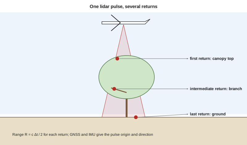
The range on its own is just a distance. To turn it into a point, the sensor must know exactly where it was and which way the beam was pointing at that instant. On a tripod, the scanner's own angle encoders give the beam direction, and the scanner position comes from control targets or from registration with other scans. On aircraft and vehicles, a GNSS receiver and an inertial measurement unit (IMU) track the sensor's position and orientation, a combination often called the positioning and orientation system, and every laser shot is combined with the trajectory computed from them. The coordinates of each point then come from the sensor position plus the range along the beam direction, after correcting for the small offsets and angles between the GNSS antenna, the IMU and the laser, which are found by calibration.
A single pulse can produce several returns. When a pulse hits a tree, part of it reflects from the top of the canopy, part from branches lower down and part from the ground underneath. Discrete-return sensors record the first, last and several intermediate returns; full-waveform sensors record the whole returning signal. This ability to see through gaps in vegetation is what makes airborne lidar so valuable for mapping the ground in forests, where photogrammetry sees only the canopy.
Each return also has an intensity, the strength of the reflected signal, which depends on the surface. Asphalt is dark and weak; road paint and retroreflective signs are bright. Intensity images look like black-and-white photographs and help in identifying features. Water absorbs the near-infrared light used by most topographic lidars, so lakes and rivers usually show as gaps; bathymetric lidar, discussed in lesson 10, uses green light that penetrates clear water.
Airborne, mobile and terrestrial lidar
| Platform | Typical range and coverage | Typical accuracy | Typical uses |
|---|---|---|---|
| Airborne (crewed aircraft) | 1,000–4,000 m above ground; hundreds of km² per day | 5–15 cm vertical | Regional terrain models, floodplains, forestry |
| Drone lidar | 40–120 m above ground; up to a few km² per day | 3–6 cm | Sites, corridors, stockpiles, small floodplains |
| Mobile (vehicle, rail, boat) | 0–100 m from the vehicle at traffic speeds | 1–5 cm with good control | Highways, rail, utilities, city streets |
| Terrestrial (tripod) | 0.5–300 m or more from the scanner | 2–6 mm | Buildings, plants, bridges, heritage, tunnels |
| Handheld and backpack | A few tens of metres, walking speed | 1–3 cm | Interiors, underground, quick as-builts |
Airborne lidar flown from crewed aircraft is the backbone of national and provincial or state elevation programmes. The aircraft flies parallel lines with a scanning mirror or rotating prism sweeping the beam from side to side, producing a swath several hundred metres to a couple of kilometres wide, with overlap between adjacent swaths to check and improve the alignment. Drone lidar brings the same principles to smaller areas at lower altitude, with higher point density but shorter flight times.
Mobile lidar mounts one or more scanners, cameras and a high-grade GNSS and IMU on a vehicle. Because GNSS can drop out under bridges, in tunnels and between tall buildings, the IMU must carry the trajectory through these gaps, and the trajectory is later adjusted to ground control targets painted or measured along the route. Mobile lidar is now standard for highway asset inventories, clearance surveys and pavement condition studies, and it keeps survey crews off busy road shoulders.
Terrestrial laser scanners sit on a tripod and sweep the beam horizontally and vertically to capture everything in view. A single scan may contain tens of millions of points. Because nothing is captured behind obstacles, a site is scanned from many positions, and the scans are joined by registration, either to targets such as spheres or checkerboards whose positions are surveyed, or by matching the overlapping surfaces directly with algorithms such as iterative closest point. Registered scans are tied to project control so that they can be combined with other survey data.
Point density and spacing
The number of points per square metre, the point density, determines what can be resolved. A density of 2 points/m² is enough for a regional bare-earth terrain model with 1 m grid cells; 8 to 20 points/m² is needed for detailed floodplain and engineering work; drone and mobile systems may deliver hundreds or thousands. The nominal pulse spacing is roughly the inverse of the square root of the density.
For a scanning airborne sensor, the density on a single swath depends on the pulse rate, the aircraft's ground speed and the swath width, which itself depends on the flying height and the scan angle. Overlap between swaths multiplies the density in the overlap areas.
where \(w\) is the swath width, \(H - h\) the height above ground, \(\theta\) the full scan angle, PRF the effective pulse repetition frequency, \(v\) the ground speed and \(\rho\) the density for a single pass. Real systems lose some pulses to water, steep surfaces and the turning of the scan mirror, so planners allow a margin.
Worked problem
Planning an airborne lidar flight for the floodplain study
The Oldman River floodplain study needs at least 8 points/m² on the ground from a single pass, with 30 per cent overlap between swaths. The sensor runs at an effective 400 kHz with a 40° full scan angle. The aircraft flies at 120 knots (61.7 m/s). Find the maximum flying height above ground.
Show solution
- \[w_{\max} = \frac{\text{PRF}}{v\,\rho} = \frac{400\,000}{61.7 \times 8} = 810\ \text{m}\]
- \[H - h = \frac{w}{2\tan 20°} = \frac{810}{2 \times 0.3640} = 1\,113\ \text{m}\]
- \[\text{line spacing} = (1 - 0.30) \times 810 = 567\ \text{m}\]
- \[\text{nominal pulse spacing} = \frac{1}{\sqrt{8}} = 0.35\ \text{m}\]
Answer: Ines plans to fly at about 1,050 m above ground for a margin, with flight lines about 540 m apart. In the overlap zones the density roughly doubles, which helps the ground classification under the riverbank trees.
Accuracy and its sources
Lidar accuracy is limited mostly by the positioning and orientation system, not by the laser range. An angular error of 0.005° in the IMU attitude is a horizontal error of about 9 cm at 1,000 m range. GNSS trajectory errors of a few centimetres pass directly into every point. Boresight misalignment, the small angle between the IMU and the laser axes, shows up as a mismatch between overlapping swaths, which calibration flights over buildings and flat areas are designed to find and remove. Range errors grow with distance, footprint size and steep incidence on sloping surfaces, and dark or wet surfaces return weak signals.
For this reason, lidar projects are always checked against ground survey points. Vertical accuracy is tested separately on open bare ground, where the result should be best, and in vegetated areas, where the ground surface is interpolated between fewer returns. Swath-to-swath differences, measured on flat hard surfaces in the overlaps, show whether the calibration is good. The ASPRS Positional Accuracy Standards and national lidar base specifications set how these tests are reported.
Classifying point clouds
A raw point cloud is just coordinates and intensities. To be useful, each point is assigned a class: ground, low, medium or high vegetation, building, water, bridge deck, wire, noise and others, following the standard classes defined for the LAS file format. Ground classification is the most important step, because it produces the bare-earth model. Algorithms typically start from the lowest points in each area and grow a surface upward, accepting points that lie close to it and rejecting points that rise too steeply. Automatic classification is then reviewed and edited by technicians, especially at stream banks, bridges, embankments and dense shrubs, where algorithms make most mistakes. Machine learning now classifies buildings, vegetation, poles and wires with growing reliability.
| Product | Made from | Typical uses |
|---|---|---|
| Digital terrain model (bare earth) | Ground-classified points | Floodplain mapping, drainage, earthworks, contours |
| Digital surface model | First returns | Line of sight, solar exposure, obstruction surveys |
| Canopy height model | DSM minus DTM | Forest inventory, vegetation clearance near power lines |
| Breaklines | Edges of water, curbs, embankments | Hydro-flattening, accurate grading models |
| Feature extraction | Classified points and intensity | Building footprints, poles, signs, wires |
Bare-earth models for flood mapping are usually hydro-flattened: water surfaces are set to a flat or smoothly falling elevation using breaklines along the banks, because the lidar returns from water are missing or unreliable. Bridges are removed from the ground surface so that the river channel flows under them in hydraulic models.
Lidar in public programmes
In Canada, provinces, municipalities and the federal government have acquired airborne lidar for flood hazard mapping, forestry and infrastructure. Natural Resources Canada coordinates lidar acquisition through the Flood Hazard Identification and Mapping Program, and publishes high-resolution elevation data through the CanElevation series. Alberta has acquired provincial lidar coverage for forestry and flood mapping, and many Alberta municipalities, including Lethbridge, maintain their own lidar and orthophoto data.
Computing density and accuracy
# Airborne lidar planning: swath, density, spacing, and the effect of attitude error
import math

def plan(prf_hz, speed_ms, agl_m, fov_deg, overlap):
    w = 2 * agl_m * math.tan(math.radians(fov_deg / 2))
    rho = prf_hz / (speed_ms * w)
    spacing = 1 / math.sqrt(rho)
    lines = (1 - overlap) * w
    return w, rho, spacing, lines

prf, v, fov = 400_000, 61.7, 40
print(" AGL (m)  swath (m)  density (pts/m2)  spacing (m)  line gap (m)")
for agl in (600, 900, 1050, 1500, 2500):
    w, rho, sp, gap = plan(prf, v, agl, fov, 0.30)
    print(f"{agl:8.0f} {w:10.0f} {rho:17.1f} {sp:12.2f} {gap:13.0f}")

# Horizontal error caused by an IMU attitude error at the edge of the swath
for err_deg in (0.002, 0.005, 0.010):
    for agl in (100, 1000):
        slant = agl / math.cos(math.radians(fov / 2))
        print(f"attitude error {err_deg:.3f} deg at {agl:4d} m AGL: {slant * math.radians(err_deg) * 100:5.1f} cm")

# Point density counted from a small sample cloud on a 1 m grid
import random
random.seed(7)
pts = [(random.uniform(0, 20), random.uniform(0, 20)) for _ in range(3400)]
cells = {}
for x, y in pts:
    cells[(int(x), int(y))] = cells.get((int(x), int(y)), 0) + 1
counts = sorted(cells.get((i, j), 0) for i in range(20) for j in range(20))
print(f"Mean density {len(pts) / 400:.1f} pts/m2, empty cells {counts.count(0)}, "
f"5th percentile {counts[len(counts) // 20]} pts per cell") AGL (m) swath (m) density (pts/m2) spacing (m) line gap (m)
600 437 14.8 0.26 306
900 655 9.9 0.32 459
1050 764 8.5 0.34 535
1500 1092 5.9 0.41 764
2500 1820 3.6 0.53 1274
attitude error 0.002 deg at 100 m AGL: 0.4 cm
attitude error 0.002 deg at 1000 m AGL: 3.7 cm
attitude error 0.005 deg at 100 m AGL: 0.9 cm
attitude error 0.005 deg at 1000 m AGL: 9.3 cm
attitude error 0.010 deg at 100 m AGL: 1.9 cm
attitude error 0.010 deg at 1000 m AGL: 18.6 cm
Mean density 8.5 pts/m2, empty cells 0, 5th percentile 4 pts per cellThe table shows the trade-off clearly: flying higher widens the swath and reduces the number of flight lines, but density falls in proportion. At 1,050 m the single-pass density is just above the 8 points/m² required. The attitude lines show why drone lidar, flying at 100 m, can tolerate a cheaper IMU than an aircraft at 1,000 m: the same angular error causes ten times less position error. The last line counts points in 1 m cells, which is how density specifications are checked in practice; they are usually stated for a percentage of cells, not only as an average, because a few gaps can matter more than the mean.
Choosing between lidar and photogrammetry
Lidar and photogrammetry overlap in what they deliver, and many projects use both. Lidar is the better choice under vegetation, for thin features such as wires, in poor light and where the surface has little texture, such as snow or fresh asphalt. Photogrammetry is cheaper for open sites, gives realistic colour and orthophotos as part of the same process, and its point clouds are very dense on textured surfaces. Coulee Geomatics flies drone photogrammetry on the open Coulee Ridge subdivision site but specifies lidar for the treed river valley and the pipeline crossings of coulees, where the ground under shrubs controls the grading and drainage design.
Common mistakes
MistakeSpecifying only average point density.
InsteadSpecify density for a percentage of cells, and the spacing of ground points under vegetation.
MistakeUsing first-return surfaces as bare ground.
InsteadUse ground-classified points and check classification in difficult areas.
MistakeTesting accuracy only on open pavement.
InsteadReport bare-ground and vegetated accuracy separately against independent check points.
MistakeIgnoring swath misalignment.
InsteadMeasure swath-to-swath differences and recalibrate boresight if they are large.
Summary and key terms
- Lidar measures range from the travel time of laser pulses: \(R = c\Delta t/2\).
- GNSS and an IMU give the sensor position and orientation for every pulse.
- Multiple returns let airborne lidar map the ground beneath vegetation.
- Density depends on pulse rate, speed and swath width; spacing is about \(1/\sqrt{\rho}\).
- Accuracy is controlled mostly by trajectory and boresight calibration.
- Point classification turns clouds into bare-earth models and features.
- Lidar
- Light detection and ranging, measuring distances with laser pulses.
- IMU
- Inertial measurement unit, which measures accelerations and rotations to track orientation.
- Return
- A reflection of a lidar pulse from a surface; one pulse can give several returns.
- Point density
- The number of lidar points per square metre.
- Registration
- Joining overlapping scans into one coordinate system.
- Boresight
- The small angular misalignment between the IMU and the laser scanner.
- Hydro-flattening
- Setting water surfaces in a terrain model to a flat or smoothly falling elevation.
Practice problems
Work each problem on paper first, then reveal the answer to check.
A pulse returns after 6.67 µs. What is the range?
Show answer
\(3\times10^8 \times 6.67\times10^{-6}/2 \approx 1\,000\) m.
A sensor at 800 m above ground has a 50° full scan angle. Find the swath width.
Show answer
\(2 \times 800 \times \tan 25° = 746\) m.
What nominal pulse spacing corresponds to 16 points/m²?
Show answer
\(1/\sqrt{16} = 0.25\) m.
An IMU has an attitude error of 0.003°. What horizontal error does this cause at 1,500 m range?
Show answer
\(1500 \times 0.003 \times \pi/180 = 7.9\) cm.
Why are bridges removed from the bare-earth model used for flood studies?
Show answer
So that the river channel can carry flow beneath them in the hydraulic model.
Lesson quiz · 5 questions
Score 60% or more to complete this lesson.
Create a free account to save your progress, take quizzes and earn a certificate.