
GEOM-200 · Lesson 3 of 12 · 20 min
Coordinate systems
Once we have a datum, we still need a way to write positions down. Geomatics engineers move constantly between several kinds of coordinates: latitude, longitude and height on the ellipsoid; three-dimensional Cartesian coordinates centred on the Earth; local east, north and up coordinates around a point of interest; and flat map grid coordinates from a projection. Each is convenient for a different job, and the conversions between them are routine operations in every GNSS receiver, GIS and design package. This lesson explains each system, shows how to convert between them, and describes how coordinate systems are labelled so that software and people do not mix them up.
Geodetic coordinates
Geodetic coordinates locate a point by its geodetic latitude \(\varphi\), longitude \(\lambda\) and ellipsoid height \(h\). Latitude is the angle between the equatorial plane and the normal to the ellipsoid at the point, positive north. Longitude is the angle in the equatorial plane east of the prime meridian through Greenwich; in North America longitudes are west, so they are negative in the usual sign convention. Ellipsoid height is the distance above the ellipsoid along the normal.
Angles can be written in degrees, minutes and seconds or in decimal degrees. One minute is 1/60 of a degree and one second is 1/3600. Because a second of latitude is about 31 m on the ground, coordinates must carry enough digits for the job: five decimal places of a degree, or about a tenth of an arc-second, gives roughly a metre; seven decimal places gives roughly a centimetre. Many data problems come from coordinates that were rounded, truncated or had their sign dropped somewhere in a chain of software.
Worked problem
Converting between degrees, minutes and seconds and decimal degrees
A control monument near Lethbridge has latitude 49°41′52.3184″ N and longitude 112°50′07.6450″ W. Convert both to signed decimal degrees.
Show solution
- \[\varphi = 49 + 41/60 + 52.3184/3600 = 49.697\,866°\]
- \[\lambda = -\Big(112 + 50/60 + 7.6450/3600\Big) = -112.835\,457°\]
Answer: West longitudes are negative in signed decimal degrees. Six decimal places are kept here, which is about 0.1 m; survey software normally keeps eight or more.
Earth-centred, Earth-fixed coordinates
For satellite positioning and for transformations between frames, a three-dimensional Cartesian system is more convenient. Earth-centred, Earth-fixed (ECEF) coordinates have their origin at the centre of the ellipsoid, the Z axis along the rotation axis toward the north pole, the X axis through the equator at the prime meridian, and the Y axis through the equator at 90° E. GNSS receivers compute positions in ECEF internally, and Helmert transformations between frames are written in ECEF. The conversion from geodetic coordinates uses the prime vertical radius \(N\) from lesson 2:
The reverse conversion, from X, Y and Z back to latitude, longitude and height, has no simple closed form because \(N\) depends on the latitude being sought. Longitude follows directly from \(\tan\lambda = Y/X\), but latitude and height are found by a short iteration or by one of several closed-form approximations that are accurate to well below a millimetre.
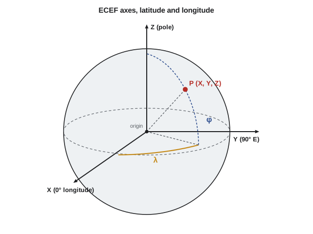
Local east, north, up coordinates
ECEF coordinates are awkward for local work: a monument in southern Alberta or Montana has X, Y and Z values in the millions of metres, and moving 10 m north changes all three. For a local view, we use a topocentric system at a chosen origin, with axes pointing east, north and up along the ellipsoid normal. This East-North-Up (ENU) system is what we mean when we say a GNSS baseline is 812 m east and 230 m north. The conversion is a rotation of the ECEF difference vector \(\Delta X, \Delta Y, \Delta Z\) between the point and the origin:
Over a few kilometres ENU coordinates behave like a flat survey grid, but they are not a map projection: the up axis is fixed at the origin, so points far away appear to drop below the horizontal plane because of the Earth's curvature. At 1 km the drop is about 8 cm, at 10 km about 8 m.
Map projections and grid coordinates
Engineering drawings, GIS layers and survey computations are much simpler on a flat grid of northings and eastings. A map projection is the mathematical rule that turns latitude and longitude into grid coordinates. No projection can flatten a curved surface without distortion, so each is designed to control the kind and amount of distortion that matters most. Conformal projections preserve angles and shapes over small areas, which is what surveying needs, at the cost of a scale that changes from place to place. Equal-area projections preserve area, which suits thematic maps of land cover or population. Others compromise.
Two conformal projections dominate in North America. The transverse Mercator projection wraps a cylinder around the Earth touching along a central meridian; it suits zones that are long north–south. The Lambert conformal conic projection uses a cone cutting the Earth along two standard parallels; it suits zones that are long east–west. The amount by which a projection stretches or shrinks distances at a point is its scale factor \(k\), and zones are kept narrow enough that \(k\) stays close to 1.
The Universal Transverse Mercator (UTM) system divides the world into 60 zones 6° of longitude wide, numbered eastward from 180°. Each zone has a central meridian scale factor of 0.9996, a false easting of 500,000 m and, in the northern hemisphere, a false northing of 0. Lethbridge lies in UTM zone 12, whose central meridian is 111° W. Alberta also defines the Alberta 3TM system, with 3° zones and a central scale factor of 0.9999, which halves the distortion across a zone and is used for many provincial datasets. Lesson 9 of CIV-250 shows how grid and ground distances are reconciled on the Coulee Ridge project.
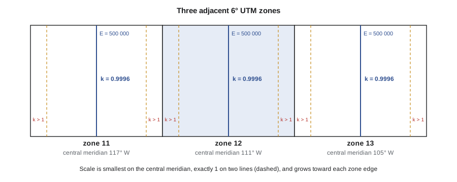
Because each zone has its own origin, coordinates in two different UTM zones, or in UTM and a provincial or state system, cannot be combined directly. A project that crosses a zone boundary either chooses one zone and accepts larger distortion at its edge, or uses a custom projection designed for the project.
Project and low-distortion coordinate systems
For construction and municipal work many organizations prefer coordinates in which grid distances equal ground distances. A low-distortion projection is a transverse Mercator or Lambert projection with its origin and scale factor chosen for the project's location and elevation, so that grid and ground distances agree to a few parts per million over the area of interest. An alternative is a ground-scaled project system, made by scaling national grid coordinates about a chosen point. Either way, the defining parameters must be published with the data so that anyone can relate project coordinates back to the national system.
Labelling coordinate reference systems
Software needs an unambiguous label for every coordinate reference system (CRS). The most widely used registry is the EPSG Geodetic Parameter Dataset, which assigns numeric codes to datums, ellipsoids, projections and complete CRSs; for example, EPSG:4326 is WGS84 latitude and longitude, used by most web maps. A complete CRS definition states the datum and its realization, the ellipsoid, the projection and its parameters, the axis order and the units. Formats such as the Well-Known Text (WKT) standard carry all of this inside data files.
Three traps catch even experienced users. First, axis order: some standards list latitude first and others longitude first, and swapping them puts Lethbridge or Great Falls somewhere in the Indian Ocean. Second, units: metres, international feet and US survey feet differ, and the US survey foot was officially retired at the end of 2022 but survives in older data. Third, epochs: two datasets in the same named frame but different epochs can differ by several centimetres or more. Coulee Geomatics's data standard requires every file to carry a full CRS definition, not just a name.
| System | Coordinates | Typical use |
|---|---|---|
| Geodetic | Latitude, longitude, ellipsoid height | Control, GNSS output, global datasets |
| ECEF | X, Y, Z from the Earth’s centre | GNSS computation, frame transformations |
| Local ENU | East, north, up from an origin | GNSS baselines, local engineering models |
| Projected grid | Northing, easting (plus elevation) | Plans, GIS, construction |
| Project / low-distortion | Northing, easting at ground scale | Municipal and construction projects |
# Geodetic <-> ECEF on GRS80, and ENU of a second point relative to a base
import math

a = 6378137.0
f = 1 / 298.257222101
e2 = 2 * f - f * f

def to_ecef(lat, lon, h):
    p, l = math.radians(lat), math.radians(lon)
    N = a / math.sqrt(1 - e2 * math.sin(p) ** 2)
    return ((N + h) * math.cos(p) * math.cos(l),
            (N + h) * math.cos(p) * math.sin(l),
            (N * (1 - e2) + h) * math.sin(p))

def to_geodetic(X, Y, Z):
    lon = math.atan2(Y, X)
    p = math.hypot(X, Y)
    lat = math.atan2(Z, p * (1 - e2))
    for _ in range(6):
        N = a / math.sqrt(1 - e2 * math.sin(lat) ** 2)
        h = p / math.cos(lat) - N
        lat = math.atan2(Z, p * (1 - e2 * N / (N + h)))
    return math.degrees(lat), math.degrees(lon), h

def enu(base, pt):
    lat0, lon0 = math.radians(base[0]), math.radians(base[1])
    X0, Y0, Z0 = to_ecef(*base)
    X, Y, Z = to_ecef(*pt)
    dX, dY, dZ = X - X0, Y - Y0, Z - Z0
    e = -math.sin(lon0) * dX + math.cos(lon0) * dY
    n = (-math.sin(lat0) * math.cos(lon0) * dX - math.sin(lat0) * math.sin(lon0) * dY
         + math.cos(lat0) * dZ)
    u = (math.cos(lat0) * math.cos(lon0) * dX + math.cos(lat0) * math.sin(lon0) * dY
         + math.sin(lat0) * dZ)
    return e, n, u

base = (49.697866, -112.835457, 895.000)       # control monument (lat, lon, h)
X, Y, Z = to_ecef(*base)
print(f"ECEF: X = {X:,.3f}  Y = {Y:,.3f}  Z = {Z:,.3f} m")
lat, lon, h = to_geodetic(X, Y, Z)
print(f"back: lat = {lat:.8f}  lon = {lon:.8f}  h = {h:.4f} m")

rover = (49.705000, -112.820000, 901.250)
e, n, u = enu(base, rover)
print(f"rover ENU from base: e = {e:.3f} m, n = {n:.3f} m, u = {u:.3f} m")
print(f"horizontal distance = {math.hypot(e, n):.3f} m")
zone = int((180 + base[1]) // 6) + 1
print(f"UTM zone {zone}, central meridian {-183 + 6 * zone} deg")ECEF: X = -1,604,397.584 Y = -3,810,109.050 Z = 4,841,802.823 m back: lat = 49.69786600 lon = -112.83545700 h = 895.0000 m rover ENU from base: e = 1115.125 m, n = 793.694 m, u = 6.103 m horizontal distance = 1368.741 m UTM zone 12, central meridian -111 deg
The round trip returns the original latitude, longitude and height to well under a millimetre, which is the test every conversion routine should pass. The rover's up value is about 0.15 m smaller than its ellipsoid height difference of 6.25 m because, over a horizontal distance of about 1.4 km, the curved ellipsoid falls away below the base's horizontal plane by roughly \(d^2/2R\). That is exactly the curvature effect described earlier, and it is why ENU coordinates are used only over short distances. The last lines compute the UTM zone from the longitude: zones are numbered from 1 at 180° W, so a longitude of about −112° or −111° falls in zone 12, whose central meridian is 111° W.
Conversions like these are built into every GNSS controller and GIS, so engineers rarely type them by hand. Knowing what they do still matters, because the most common data errors are not arithmetic mistakes but wrong inputs: a height entered as an orthometric height when the routine expects ellipsoid height, a longitude without its sign, or a datum assumed rather than checked. A quick round-trip test or a plot against a known point catches most of them in seconds.
Common mistakes
MistakeDropping the minus sign on west longitudes.
InsteadUse signed decimal degrees and check that points plot in the right place before using them.
MistakeMixing coordinates from two projection zones or two systems.
InsteadTransform everything into one CRS and record which one.
MistakeSwapping latitude and longitude order.
InsteadCheck the axis order of each format and software package.
MistakeLabelling a dataset with only a datum name.
InsteadGive the full CRS: datum realization, epoch, projection, axis order and units, ideally with an EPSG code or WKT.
Summary and key terms
- Geodetic coordinates are latitude, longitude and ellipsoid height on a stated datum.
- ECEF coordinates are Cartesian X, Y, Z from the Earth's centre and are used inside GNSS and frame transformations.
- Local ENU coordinates rotate ECEF differences to east, north and up at an origin.
- Map projections give flat grid coordinates; conformal projections such as transverse Mercator and Lambert conformal conic preserve angles.
- UTM zones are 6° wide with a central scale factor of 0.9996; provincial and state systems use narrower zones.
- Every dataset needs a full coordinate reference system definition, including axis order, units and epoch.
- Geodetic latitude
- The angle between the equatorial plane and the normal to the ellipsoid at a point.
- ECEF
- Earth-centred, Earth-fixed Cartesian coordinates with origin at the Earth’s centre.
- ENU
- Local east, north and up coordinates relative to a chosen origin.
- Conformal projection
- A map projection that preserves angles and local shapes.
- Scale factor
- The ratio of a distance on the projection to the corresponding distance on the ellipsoid.
- Coordinate reference system
- A complete definition of how coordinates relate to the Earth, including datum, projection, axes and units.
- EPSG code
- A numeric identifier for a coordinate reference system or component in the EPSG registry.
Practice problems
Work each problem on paper first, then reveal the answer to check.
Convert 51°02′45″ N to decimal degrees.
Show answer
\(51 + 2/60 + 45/3600 = 51.045\,833°\).
Convert −114.0719° to degrees, minutes and seconds.
Show answer
114°04′18.8″ W.
In which UTM zone is longitude −104.6°?
Show answer
Zone \(\lfloor(180 - 104.6)/6\rfloor + 1 = 13\).
Roughly how far does a horizontal plane drop below the Earth's surface 5 km from its origin?
Show answer
About \(d^2/(2R) = 25\,000\,000/12\,742\,000 \approx 2.0\) m.
Why are ECEF coordinates used for frame transformations?
Show answer
The Helmert transformation is a simple 3D rotation, translation and scale of Cartesian coordinates.
Lesson quiz · 5 questions
Score 60% or more to complete this lesson.
Create a free account to save your progress, take quizzes and earn a certificate.